

i
i
i
i
i
i
i
i
116 6. Transformation Matrices
(0,1)
(.866,.5)
(.5,.866)
(1,0)
Figure 6.7. A rotation by minus thirty degrees. Note that the rotation is clockwise and that
cos(-30
◦
) ≈ .866 and sin(-30
◦
)=-.5.
Because the norm of each row of a rotation matrix is one (sin
2
φ+cos
2
φ =1),
and the rows are orthogonal (cos φ(−sin φ)+sinφ cos φ =0), we see that ro-
tation matrices are orthogonal matrices (Section 5.2.4). By looking at the matrix
we can read off two pairs of orthonormal vectors: the two columns, which are the
vectors to which the transformation sends the canonical basis vectors (1, 0) and
(0, 1); and the rows, which are the vectors that the transformations sends to the
canonical basis vectors.
Said briefly, Re
i
= u
i
and
Rv
i
= u
i
, for a rotation with
columns u
i
and rows v
i
.
6.1.4 Reflection
We can reflect a vector across either of the coordinate axes by using a scale with
one negative scale factor (see Figures 6.8 and 6.9):
reflect-y =
−10
01
, reflect-x =
10
0 −1
.
Figure 6.8. A reflection about the
y
-axis is achieved by multiplying all
x
-coordinates by -1.
i
i
i
i
i
i
i
i
6.1. 2D Linear Transformations 117
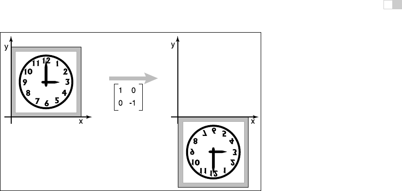
Figure 6.9. A reflection about the
x
-axis is achieved by multiplying all
y
-coordinates by -1.
While one might expect that the matrix with −1 in both elements of the diagonal
is also a reflection, in fact it is just a rotation by π radians.
This rotation can also be
called a “reflection through
the origin.”
6.1.5 Composition and Decomposition of Transformations
It is common for graphics programs to apply more than one transformation to an
object. For example, we might want to first apply a scale S, and then a rotation
R. This would be done in two steps on a 2D vector v
1
:
first,v
2
= Sv
1
, then,v
3
= Rv
2
.
Another way to write this is
v
3
= R (Sv
1
) .
Because matrix multiplication is associative, we can also write
v
3
=(RS) v
1
.
In other words, we can represent the effects of transforming a vector by two ma-
trices in sequence using a single matrix of the same size, which we can compute
by multiplying the two matrices: M = RS (Figure 6.10).
It is very important to remember that these transforms are applied from the
right side first. So the matrix M = RS first applies S and then R.

i
i
i
i
i
i
i
i
118 6. Transformation Matrices
x
1.0 0
0 0.5
y
x
y
x
y
.707 -707
.707 .707
.707 -.353
.707 .353
Figure 6.10. Applying the two transform matrices in sequence is the same as applying the
product of those matrices once. This is a key concept that underlies most graphics hardware
and software.
Example. Suppose we want to scale by one-half in the vertical direction and then
rotate by π/4 radians (45 degrees). The resulting matrix is
0.707 −0.707
0.707 0.707
10
00.5
=
0.707 −0.353
0.707 0.353
.
It is important to always remember that matrix multiplication is not commutative.
So the order of transforms does matter. In this example, rotating first, and then
scaling, results in a different matrix (see Figure 6.11):
10
00.5
0.707 −0.707
0.707 0.707
=
0.707 −0.707
0.353 0.353
.
Example. Using the scale matrices we have presented, nonuniform scaling can
only be done along the coordinate axes. If we wanted to stretch our clock by
50% along one of its diagonals, so that 8:00 through 1:00 move to the northwest
and 2:00 through 7:00 move to the southeast, we can use rotation matrices in
combination with an axis-aligned scaling matrix to get the result we want. The
idea is to use a rotation to align the scaling axis with a coordinate axis, then
scale along that axis, then rotate back. In our example, the scaling axis is the
“backslash” diagonal of the square, and we can make it parallel to the x-axis with
i
i
i
i
i
i
i
i
6.1. 2D Linear Transformations 119
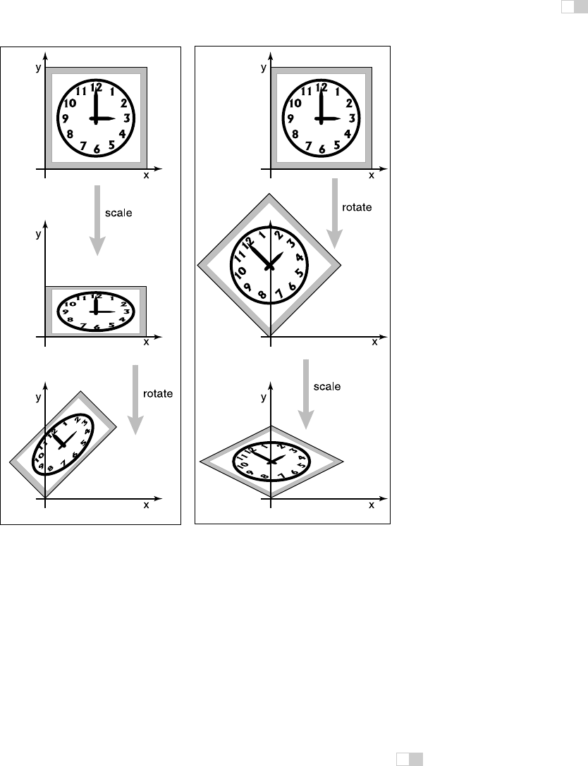
Figure 6.11. The order in which two transforms are applied is usually important. In this
example, we do a scale by one-half in
y
and then rotate by 45
◦
. Reversing the order in which
these two transforms are applied yields a different result.
a rotation by +45
◦
. Putting these operations together, the full transformation is
rotate(−45
◦
) scale(1.5, 1) rotate(45
◦
).
Remember to read the
transformations from right
to left.
In mathematical notation, this can be written RSR
T
. The result of multiply-
ing the three matrices together is
It is no coincidence that
this matrix is symmetric—
try applying the transpose-
of-product rule to the for-
mula RSR
T
.
1.25 −0.25
−0.25 1.25
i
i
i
i
i
i
i
i
120 6. Transformation Matrices
Building up a transformation from rotation and scaling transformations actu-
ally works for any linear transformation at all, and this fact leads to a powerful
way of thinking about these transformations, as explored in the next section.
6.1.6 Decomposition of Transformations
Sometimes it’s necessary to “undo” a composition of transformations, taking a
transformation apart into simpler pieces. For instance, it’s often useful to present
a transformation to the user for manipulation in terms of separate rotations and
scale factors, but a transformation might be represented internally simply as a
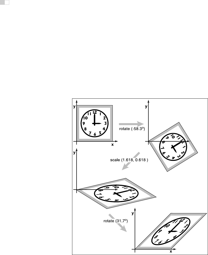
Figure 6.12. Singular Value Decomposition (SVD) for a shear matrix. Any 2D matrix can
be decomposed into a product of rotation, scale, rotation. Note that the circular face of the
clock must become an ellipse because it is just a rotated and scaled circle.
..................Content has been hidden....................
You can't read the all page of ebook, please click here login for view all page.