
Whether dealing with local of global data, geographical maps are a suitable visualization. To plot data on a map, we need coordinates, usually in the form of latitude and longitude values. Several file formats exist with which we can save geographical data. In this recipe, we will use the special shapefile format and the more common tab separated values (TSV) format. The shapefile format was created by the Esri company and uses three mandatory files with the extensions .shp , .shx , and .dbf. The .dbf file contains a database with extra information for each geographical location in the shapefile. The shapefile we will use contains information about country borders, population, and
Gross Domestic Product (GDP). We can download the shapefile with the cartopy library. The TSV file holds population data for more than 4000 cities as a timeseries. It comes from https://nordpil.com/resources/world-database-of-large-cities/ (retrieved July 2015).
First, we need to install Proj.4 from source or, if you are lucky, using a binary distribution from https://github.com/OSGeo/proj.4/wiki (retrieved July 2015). The instructions to install Proj.4 are available at https://github.com/OSGeo/proj.4 (retrieved July 2015). Then, install cartopy with pip—I wrote the code with cartopy-0.13.0. Alternatively, we can run the following command:
$ conda install -c scitools cartopy
- The imports are as follows:
import cartopy.crs as ccrs
import matplotlib.pyplot as plt
import cartopy.io.shapereader as shpreader
import matplotlib as mpl
import pandas as pd
from dautil import options
from dautil import data
- We will use color to visualize country populations and populous cities. Load the data as follows:
countries = shpreader.natural_earth(resolution='110m', category='cultural', name='admin_0_countries') cities = pd.read_csv(data.Nordpil().load_urban_tsv(), sep=' ', encoding='ISO-8859-1') mill_cities = cities[cities['pop2005'] > 1000] - Draw a map, a corresponding colorbar, and mark populous cities on the map with the following code:
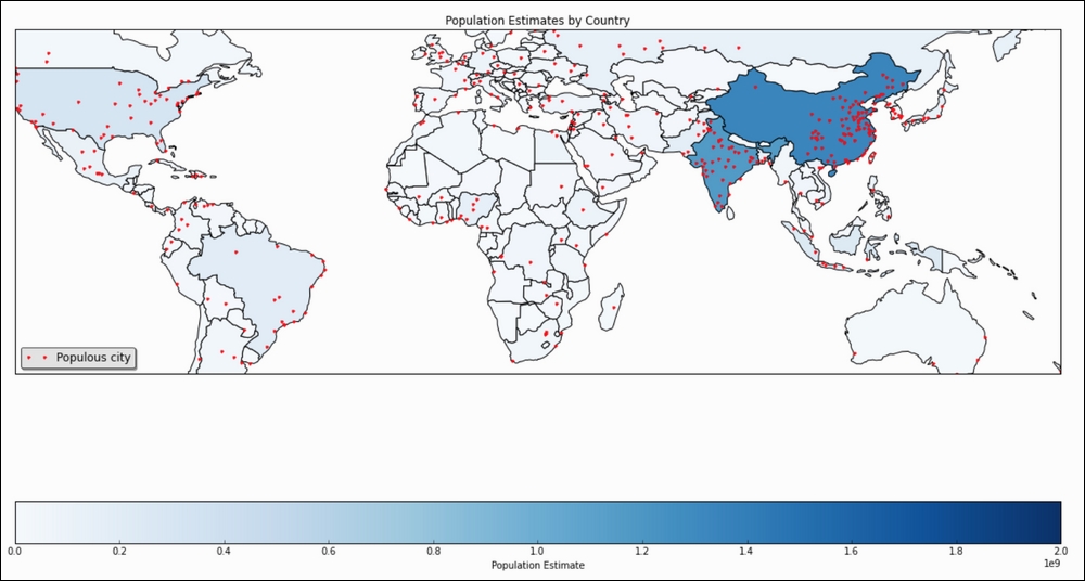
%matplotlib inline
plt.figure(figsize=(16, 12))
gs = mpl.gridspec.GridSpec(2, 1,
                           height_ratios=[20, 1])
ax = plt.subplot(gs[0], projection=ccrs.PlateCarree())

norm = mpl.colors.Normalize(vmin=0, vmax=2 * 10 ** 9)
cmap = plt.cm.Blues
ax.set_title('Population Estimates by Country')

for country in shpreader.Reader(countries).records():
    ax.add_geometries(country.geometry, ccrs.PlateCarree(),
                      facecolor=cmap(
                          norm(country.attributes['pop_est'])))

plt.plot(mill_cities['Longitude'],
         mill_cities['Latitude'], 'r.',
         label='Populous city',
         transform=ccrs.PlateCarree())

options.set_mpl_options()
plt.legend(loc='lower left')

cax = plt.subplot(gs[1])
cb = mpl.colorbar.ColorbarBase(cax,
                               cmap=cmap,
                               norm=norm,
                               orientation='horizontal')

cb.set_label('Population Estimate')
plt.tight_layout()
Refer to the following plot for the end result:
You can find the code in the plot_map.ipynb file in this book's code bundle.