The examples so far have been of continuous variables. However, other variables are discrete and can be of a binary type. Some common examples of discrete binary variables are if it is snowing in a city on a given day or not, if a patient is carrying a virus or not, and so on. One of the main differences between binary logistic and linear regression is that in binary logistic regression, we are fitting the probability of an outcome given a measured (discrete or continuous) variable, while linear regression models deal with characterizing the dependency of two or more continuous variables on each other. Logistic regression gives the probability of an occurrence given some observed variable(s). Probability is sometimes expressed as P(Y|X) and read as Probability that the value is Y given the variable X.

Algorithms that guess the discrete outcome are called classification algorithms and are a part of machine learning techniques, which will be covered later in the book.

The logistic regression model can be expressed as follows:

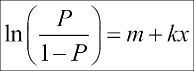
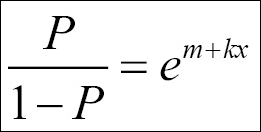
Solving this equation for P, we get the logistic probability:

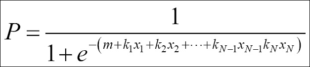
We can, just as with linear regression, add several dimensions (dependent variables) to the problem:

To illustrate what this function looks like and the difference from fitting a linear model, we plot both functions:

k = 1. 
m = -5. 
y = lambda x: k*x + m 
#p = lambda x: np.exp(k*x+m) / (1+np.exp(k*x+m)) 
p = lambda x: 1 / (1+np.exp(-1*(k*x+m))) 
 
xx = np.linspace(0,10) 
plt.plot(xx,y(xx), label='linear') 
plt.plot(xx,p(xx), label='logistic') 
plt.plot([0,abs(m)], [0.5,0.5], dashes=(4,4), color='.7') 
plt.plot([abs(m),abs(m)], [-.1,.5], dashes=(4,4), color='.7') 
 
# limits, legends and labels 
plt.ylim((-.1,1.1)) 
plt.legend(loc=2) 
plt.ylabel('P') 
plt.xlabel('xx') 

As is clearly seen, the S-shaped curve, our logistic fitting function (more generally called sigmoid function), can illustrate binary logistic probabilities much better. Playing around with k and m, we quickly realize that k determines the steepness of the slope and m moves the curve left or right. We also notice that P(Y|xx=5) = 0.5, that is, at xx=5, the outcome Y (corresponding to P=1) has a 50% probability.

Imagine that we asked students how long they studied for an exam. Can we check how long you need to study to be fairly sure to pass? To investigate this, we need to use logistic regression. It is only possible to pass or fail an exam, that is, it is a binary variable. First, we need to create the data:

studytime=[0,0,1.5,2,2.5,3,3.5,4,4,4,5.5,6,6.5,7,7,8.5,9,9,9,10.5,10.5,12,12,12,12.5,13,14,15,16,18] 
passed=[0,0,0,0,0,0,0,0,0,0,0,1,0,1,1,0,1,1,0,1,1,1,1,1,1,1,1,1,1,1] 
data = pd.DataFrame(data=np.array([studytime, passed]).T, columns=['Time', 
                    'Pass']) 
data.Time.hist(bins=6) 
plt.xlabel('Time') 
plt.ylabel('No. students'), 

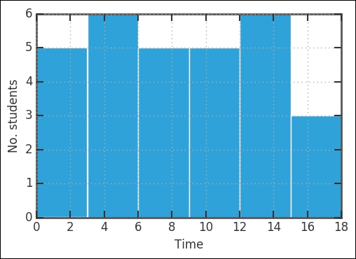
The first thing plotted is the histogram of how much time the students spent studying for the exam. It seems like it is a rather flat distribution. Here, we will check how they did on the exam:

plt.plot(data.Time, data.Pass,'o', mew=0, ms=7,) 
plt.ylim(-.1,1.1) 
plt.xlim(-0.2,16.2) 
plt.xlabel('Time studied') 
plt.ylabel('Pass? (0=no, 1=yes)'), 

This plot will now show you how much time someone studied and the outcome of the exam-if they passed given by a value of 1.0 (yes) or if they failed given by a value of 0.0 (no). The x axis goes from 0 hours (a student who did not study at all) up to 18 hours (a student who studied more).

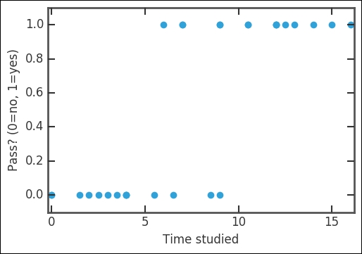
By simply inspecting the figure, it seems like sometime between 5-10 hours is needed to at least pass the exam. Once again, we use statsmodels to fit the data with our model. In statsmodels, there is a logit function that performs logistic regression:

import statsmodels.api as sm 
probfit = sm.Logit(data.Pass, sm.add_constant(data.Time, prepend=True)) 

The optimization worked; if there would have been any problems converging, error messages would have been printed instead. After running the fit, checking the summary is a good idea:

fit_results = probfit.fit() 
print(fit_results.summary()) 

The const variable is the intercept, that is, k of the fit-function, and Time is the intercept, m. The covariance parameters can be used to estimate the standard deviation by taking the square root of the diagonal of the covariance matrix:

logit_pars = fit_results.params 
intercept_err, slope_err = np.diag(fit_results.cov_params())**.5 
fit_results.cov_params() 

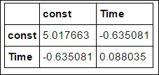
However, statsmodels also gives the uncertainty in the parameters, as can be seen from the fit summary output:

intercept = logit_pars['const'] 
slope = logit_pars['Time'] 
print(intercept,slope)
-5.79798670884 0.801979232718

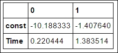
It is also possible to print out the confidence intervals directly:

fit_results.conf_int() 

Now it is appropriate to plot the fit on top of the data. We have estimated the parameters of the fit function:

plt.plot(data.Time, data.Pass,'o', mew=0, ms=7, label='Data') 
p = lambda x,k,m: 1 / (1+np.exp(-1*(k*x+m))) 
xx = np.linspace(0,data.Time.max()) 
l1 = plt.plot(xx, p(xx,slope,intercept), label='Fit') 
plt.fill_between(xx, p(xx,slope+slope_err**2, intercept+intercept_err), p(xx,slope-slope_err**2, intercept-intercept_err), alpha=0.15, color=l1[0].get_color()) 
plt.ylim(-.1,1.1) 
plt.xlim(-0.2,16.2) 
plt.xlabel('Time studied') 
plt.ylabel('Pass? (0=no, 1=yes)') 
plt.legend(loc=2, numpoints=1); 

Here, we have not only plotted the best fit curve, but also the curve corresponding to one standard deviation away. The uncertainty encompasses a lot of values. Now, with the estimated parameters, it is possible to calculate how long should we study for a 50% chance of success:

target=0.5 
x_prob = lambda p,k,m: (np.log(p/(1-p))-m)/k 
T_max = x_prob(target, slope-slope_err, intercept-intercept_err) 
T_min = x_prob(target, slope+slope_err, intercept+intercept_err) 
T_best = x_prob(target, slope, intercept) 
print('{0}% sucess rate: {1:.1f} +{2:.1f}/-    {3:.1f}'.format(int(target*100),T_best,T_max-T_best,T_best-T_min))
50% success rate: 7.2 +8.7/-4.0

So studying for 7.2 hours for this test, the chance of passing is about 50%. The uncertainty is rather large, and the 50% chance of passing could also be for about 15 hours of studying or as little as three hours. Of course, there is more to studying for an exam than the absolute number of hours put in. However, by not studying at all, the chances of passing are very slim.