Strength in numbers is the reason why large countries tend to be more successful than small countries. That doesn't mean that a person in a large country has a better life. But for the big picture, the individual person doesn't matter that much, just like in an ensemble of decision trees the results of a single tree can be ignored if we have enough trees.

In the context of classification, we define weak learners as learners that are just a little better than a baseline such as randomly assigning classes. Although weak learners are weak individually, like ants, together they can do amazing things just like ants can.

It makes sense to take into account the strength of each individual learner using weights. This general idea is called boosting. There are many boosting algorithms, of which we will use AdaBoost in this recipe. Boosting algorithms differ mostly in their weighting scheme.

AdaBoost uses a weighted sum to produce the final result. It is an adaptive algorithm that tries to boost the results for individual training examples. If you have studied for an exam, you may have applied a similar technique by identifying the type of questions you had trouble with and focusing on the difficult problems. In the case of AdaBoost, boosting is done by tweaking the weak learners.

How to do it...

The program is in the boosting.ipynb file in this book's code bundle:

1. The imports are as follows:

   import ch9util
   from sklearn.grid_search import GridSearchCV
   from sklearn.ensemble import AdaBoostRegressor
   from sklearn.tree import DecisionTreeRegressor
   import numpy as np
   import dautil as dl
   from IPython.display import HTML

2. Load the data and create an AdaBoostRegressor class:

   X_train, X_test, y_train, y_test = ch9util.temp_split()
   params = {
       'loss': ['linear', 'square', 'exponential'],
       'base_estimator__min_samples_leaf': [1, 2]
   }
   reg = AdaBoostRegressor(base_estimator=DecisionTreeRegressor(random_state=28),
                           random_state=17)

3. Grid search, fit, and predict as follows:

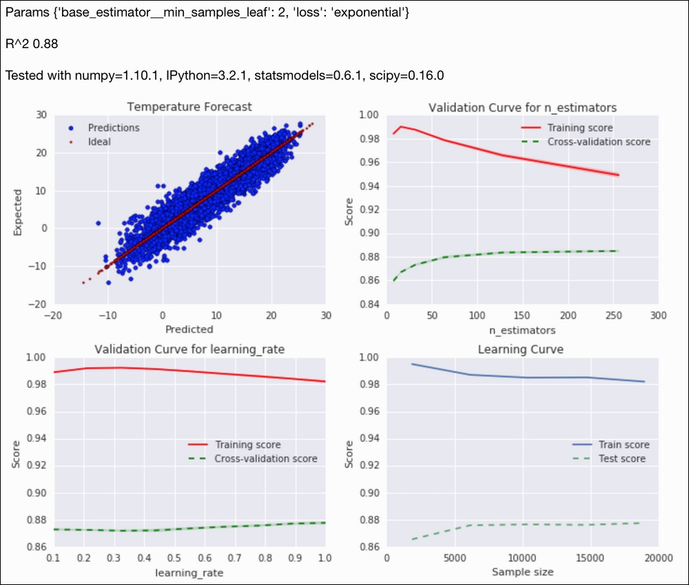
   gscv = GridSearchCV(estimator=reg,
                       param_grid=params, cv=5, n_jobs=-1)
   gscv.fit(X_train, y_train)
   preds = gscv.predict(X_test)

4. Scatter plot the predictions against the actual values:

   sp = dl.plotting.Subplotter(2, 2, context)
   html = ch9util.scatter_predictions(preds, y_test, gscv.best_params_,  
                                      gscv.best_score_, sp.ax)

5. Plot a validation curve for a range of ensemble sizes:

   nestimators = 2 ** np.arange(3, 9)
   ch9util.plot_validation(sp.next_ax(), gscv.best_estimator_, 
                           X_train, y_train, 'n_estimators', nestimators)

6. Plot a validation curve for a range of learning rates:

   learn_rate = np.linspace(0.1, 1, 9)
   ch9util.plot_validation(sp.next_ax(), gscv.best_estimator_, 
                           X_train, y_train, 'learning_rate', learn_rate)

7. Plot the learning curve as follows:

   ch9util.plot_learn_curve(sp.next_ax(), gscv.best_estimator_, 
                            X_train, y_train)
   HTML(html + sp.exit())

Refer to the following screenshot for the end result: