We discussed the issue of outliers in the context of regression elsewhere in this book (refer to the See also section at the end of this recipe). The issue is clear—the outliers make it difficult to properly fit our models. The RANdom SAmple Consensus algorithm (RANSAC) does a best effort attempt to fit our data in an iterative manner. RANSAC was introduced by Fishler and Bolles in 1981.

We often have some knowledge about our data, for instance the data may follow a normal distribution. Or, the data may be a mix produced by multiple processes with different characteristics. We could also have abnormal data due to glitches or errors in data transformation. In such cases, it should be easy to identify outliers and deal with them appropriately. The RANSAC algorithm doesn't know your data, but it also assumes that there are inliers and outliers.

The algorithm goes through a fixed number of iterations. The object is to find a set of inliers of specified size (consensus set).

RANSAC performs the following steps:

The scikit-learn RANSACRegressor class can use a suitable estimator for fitting. We will use the default LinearRegression estimator. We can also specify the minimum number of samples for fitting, the residuals threshold, a decision function for outliers, a function that decides whether a model is valid, the maximum number of iterations, and the required number of inliers in the consensus set.

How to do it...

The code is in the fit_ransac.ipynb file in this book's code bundle:

1. The imports are as follows:

   import ch9util
   from sklearn import linear_model
   from sklearn.grid_search import GridSearchCV
   import numpy as np
   import dautil as dl
   from IPython.display import HTML

2. Load the data and do a temperature prediction as follows:

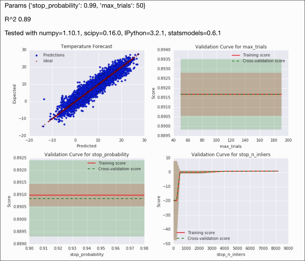
   X_train, X_test, y_train, y_test = ch9util.temp_split()
   ransac = linear_model.RANSACRegressor(random_state=27)
   params = {
       'max_trials': [50, 100, 200],
       'stop_probability': [0.98, 0.99]
   }
   
   gscv = GridSearchCV(estimator=ransac, param_grid=params, cv=5)
   gscv.fit(X_train, y_train)
   preds = gscv.predict(X_test)

3. Scatter plot the predictions against the actual values:

   sp = dl.plotting.Subplotter(2, 2, context)
   html = ch9util.scatter_predictions(preds, y_test, gscv.best_params_,
                                      gscv.best_score_, sp.ax)

4. Plot a validation curve for a range of trial numbers:

   trials = 10 * np.arange(5, 20)
   ch9util.plot_validation(sp.next_ax(), gscv.best_estimator_, 
                           X_train, y_train, 'max_trials', trials)

5. Plot a validation curve for a range of stop probabilities:

   probs = 0.01 * np.arange(90, 99)
   ch9util.plot_validation(sp.next_ax(), gscv.best_estimator_, 
                           X_train, y_train, 'stop_probability', probs)

6. Plot a validation curve for a range of consensus set sizes:

   ninliers = 2 ** np.arange(4, 14)
   ch9util.plot_validation(sp.next_ax(), gscv.best_estimator_, 
                           X_train, y_train, 'stop_n_inliers', ninliers)
   HTML(html + sp.exit())

Refer to the following screenshot for the end result: