The efficient-market hypothesis (EMH) stipulates that you can't, on average, "beat the market" by picking better stocks or timing the market. According to the EMH, all information about the market is immediately available to every market participant in one form or another, and it is immediately reflected in asset prices, so investing is like playing a game of cards with all the cards revealed. The only way you can win is by betting on very risky stocks and getting lucky.

The French mathematician Bachelor developed a test for the EMH around 1900. The test examines consecutive occurrences of negative and positive price changes. We don't count events during which the price didn't change and only use them to end a run. These types of events are relatively rare anyway for liquid markets.

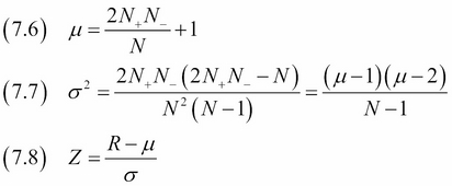
The statistical test itself is known outside finance and goes by the name of the Wald-Wolfowitz runs test. If we denote positive changes with '+' and negative changes with '-', we can have the sequence '++++−−−+++−−++++++' with 5 runs. The following equations for the mean μ (7.6), standard deviation σ (7.7), and z-score Z (7.8) of the number of runs R also require the number of negative changes N-, positive changes N+, and total number of changes N:

We assume that the number of runs follow a normal distribution, which gives us a way to potentially reject the randomness of runs at a confidence level of our choosing.

How to do it...

Have a look at the non_parametric.ipynb file in this book's code bundle.

1. The imports are as follows:

   import dautil as dl
   import numpy as np
   import pandas as pd
   import ch7util
   import matplotlib.pyplot as plt
   from scipy.stats import norm
   from IPython.display import HTML

2. Define the following function to count the number of runs:

   def count_runs(signs):
       nruns = 0
       prev = None
   
       for s in signs:
           if s != 0 and s != prev:
               nruns += 1
   
           prev = s
   
       return nruns

3. Define the following function to calculate the mean, standard deviation, and z-score:

   def proc_runs(symbol):
       ohlc = dl.data.OHLC()
       close = ohlc.get(symbol)['Adj Close'].values
       diffs = np.diff(close)
       nplus = (diffs > 0).sum()
       nmin = (diffs < 0).sum()
       n = nplus + nmin
       mean = (2 * (nplus * nmin) / n) + 1
       var = (mean - 1) * (mean - 2) / (n - 1)
       std = np.sqrt(var)
       signs = np.sign(diffs)
       nruns = count_runs(np.diff(signs))
   
       return mean, std, (nruns - mean) / std

4. Calculate the metrics for our stocks:

   means = []
   stds = []
   zscores = []
   
   for symbol in ch7util.STOCKS:
       mean, std, zscore = proc_runs(symbol)
       means.append(mean)
       stds.append(std)
       zscores.append(zscore)

5. Plot the z-scores with a line indicating the 95% confidence level:

   sp = dl.plotting.Subplotter(2, 1, context)
   dl.plotting.plot_text(sp.ax, means, stds, ch7util.STOCKS, add_scatter=True)
   sp.label()
   
   dl.plotting.bar(sp.next_ax(), ch7util.STOCKS, zscores)
   sp.ax.axhline(norm.ppf(0.95), label='95 % confidence level')
   sp.label()
   HTML(sp.exit())

Refer to the following screenshot for the end result: