
We can apply many techniques to analyze audio, and, therefore, we can debate at length about which techniques are most appropriate. The most obvious method is purportedly the FFT. As a variation, we can use the short-time Fourier transform (STFT). The STFT splits the signal in the time domain into equal parts, and it then applies the FFT to each segment. Another algorithm we will use is the cepstrum, which was originally used to analyze earthquakes but was later successfully applied to speech analysis. The power cepstrum is given by the following equation:

The algorithm is as follows:
- Calculate the Fourier transform.
- Compute the squared magnitude of the transform.
- Take the logarithm of the previous result.
- Apply the inverse Fourier transform.
- Calculate the squared magnitude again.
The cepstrum is, in general, useful when we have large changes in the frequency domain. An important use case of the cepstrum is to form feature vectors for audio classification. This requires a mapping from frequency to the mel scale (refer to the Wikipedia page mentioned in the See also section).
- The imports are as follows:
import dautil as dl
import matplotlib.pyplot as plt
import numpy as np
from ch6util import read_wav
from IPython.display import HTML
- Define the following function to calculate the magnitude of the signal with FFT:
def amplitude(arr): return np.abs(np.fft.fft(arr)) - Load the data as follows:
rate, audio = read_wav()
- Plot the audio waveform:
sp = dl.plotting.Subplotter(2, 2, context)
t = np.arange(0, len(audio)/float(rate), 1./rate)
sp.ax.plot(t, audio)
freqs = np.fft.fftfreq(audio.size, 1./rate)
indices = np.where(freqs > 0)[0]
sp.label()
- Plot the amplitude spectrum:
magnitude = amplitude(audio)
sp.next_ax().semilogy(freqs[indices], magnitude[indices])
sp.label()
- Plot the cepstrum as follows:
cepstrum = dl.ts.power(np.fft.ifft(np.log(magnitude ** 2)))
sp.next_ax().semilogy(cepstrum)
sp.label()
- Plot the STFT as a contour diagram:
npieces = 200
stft_amps = []

for i, c in enumerate(dl.collect.chunk(audio[: npieces ** 2], len(audio)/npieces)):
    amps = amplitude(c)
    stft_amps.extend(amps)

stft_freqs = np.linspace(0, rate, npieces)
stft_times = np.linspace(0, len(stft_amps)/float(rate), npieces)
sp.next_ax().contour(stft_freqs/rate, stft_freqs,
           np.log(stft_amps).reshape(npieces, npieces))
sp.label()

HTML(sp.exit())
Refer to the following screenshot for the end result:
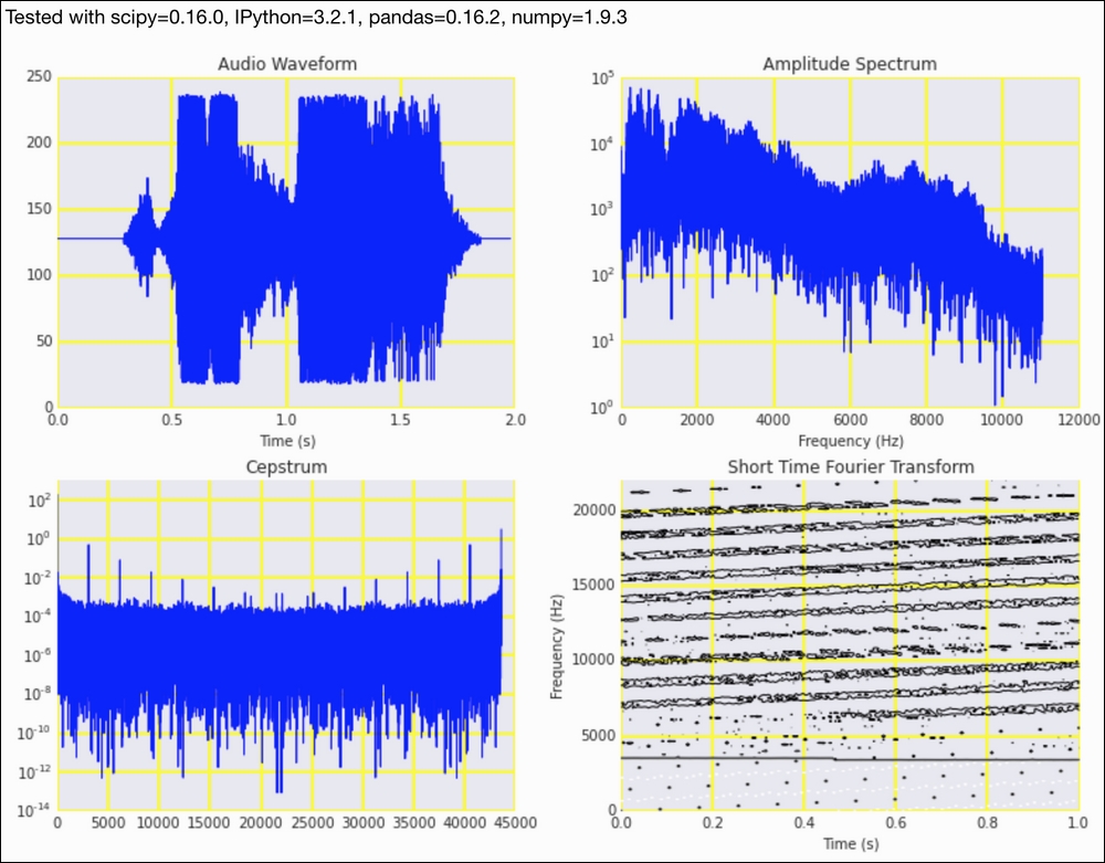
The example code is in the analyzing_audio.ipynb file in this book's code bundle.
- The Wikipedia page about the STFT at https://en.wikipedia.org/wiki/Short-time_Fourier_transform (retrieved September 2015)
- The Wikipedia page about the cepstrum at https://en.wikipedia.org/wiki/Cepstrum (retrieved September 2015)
- The Wikipedia page about the mel scale at https://en.wikipedia.org/wiki/Mel_scale (retrieved September 2015)