Time Series Concepts, Representations, and Models

SERGIO M. FOCARDI, PhD

Partner, The Intertek Group

FRANK J. FABOZZI, PhD, CFA, CPA

Professor of Finance, EDHEC Business School

In this entry, we introduce models of discrete-time stochastic processes (that is, time series). In financial modeling, both continuous-time and discrete-time models are used. In many instances, continuous-time models allow simpler and more concise expressions as well as more general conclusions, though at the expense of conceptual complication. For instance, in the limit of continuous time, apparently simple processes such as white noise cannot be meaningfully defined. The mathematics of asset management tends to prefer discrete-time processes, while the mathematics of derivatives tends to prefer continuous-time processes.

The first issue to address in financial econometrics is the spacing of discrete points of time. An obvious choice is regular, constant spacing. In this case, the time points are placed at multiples of a single time interval: t = i Δt. For instance, one might consider the closing prices at the end of each day. The use of fixed spacing is appropriate in many applications. Spacing of time points might also be irregular but deterministic. For instance, weekends introduce irregular spacing in a sequence of daily closing prices. These questions can be easily handled within the context of discrete-time series.

In this entry, we discuss only time series at discrete and fixed intervals of time, introducing concepts, representations, and models of time series.1

CONCEPTS OF TIME SERIES

A time series is a collection of random variables Xt indexed with a discrete time index t = …−2, −1,0,1,2, …. The variables Xt are defined over a probability space (Ω, P, ), where Ω is the set of states, P is a probability measure, and is the σ-algebra of events, equipped with a discrete filtration {t} that determines the propagation of information (see the Appendix). A realization of a time series is a countable sequence of real numbers, one for each time point.

The variables Xt are characterized by finite-dimensional distributions as well as by conditional distributions, Fs(xs/t), s > t. The latter are the distributions of the variable x at time s given the σ-algebra {t} at time t. Note that conditioning is always conditioning with respect to a σ-algebra though we will not always strictly use this notation and will condition with respect to the value of variables, for instance:

If the series starts from a given point, initial conditions must be fixed. Initial conditions might be a set of fixed values or a set of random variables. If the initial conditions are not fixed values but random variables, one has to consider the correlation between the initial values and the random shocks of the series. A usual assumption is that the initial conditions and the random shocks of the series are statistically independent.

How do we describe a time series? One way to describe a time series is to determine the mathematical form of the conditional distribution. This description is called an autopredictive model because the model predicts future values of the series from past values. However, we can also describe a time series as a function of another time series. This is called an explanatory model as one variable is explained by another. The simplest example is a regression model where a variable is proportional to another exogenously given variable plus a constant term. Time series can also be described as random fluctuations or adjustments around a deterministic path. These models are called adjustment models. Explanatory, autopredictive, and adjustment models can be mixed in a single model. The data generation process (DGP) of a series is a mathematical process that computes the future values of the variables given all information known at time t.

An important concept is that of a stationary time series. A series is stationary in the “strict sense” if all finite dimensional distributions are invariant with respect to a time shift. A series is stationary in a “weak sense” if only the moments up to a given order are invariant with respect to a time shift. In this entry, time series will be considered (weakly) stationary if the first two moments are time-independent. Note that a stationary series cannot have a starting point but must extend over the entire infinite time axis. Note also that a series can be strictly stationary (i.e., have all distributions time-independent, but the moments might not exist). Thus a strictly stationary series is not necessarily weakly stationary.

A time series can be univariate or multivariate. A multivariate time series is a time-dependent random vector. The principles of modeling remain the same but the problem of estimation might become very difficult given the large numbers of parameters to be estimated.

Models of time series are essential building blocks for financial forecasting and, therefore, for financial decision-making. In particular asset allocation and portfolio optimization, when performed quantitatively, are based on some model of financial prices and returns. This entry lays down the basic financial econometric theory for financial forecasting. We will introduce a number of specific models of time series and of multivariate time series, presenting the basic facts about the theory of these processes. We will consider primarily models of financial assets, though most theoretical considerations apply to macroeconomic variables as well. These models include:

• Correlated random walks. The simplest model of multiple financial assets is that of correlated random walks. This model is only a rough approximation of equity price processes and presents serious problems of estimation in the case of a large number of processes.
• Factor models. Factor models address the problem of estimation in the case of a large number of processes. In a factor model there are correlations only among factors and between each factor and each time series. Factors might be exogenous or endogenously modeled.
• Cointegrated models. In a cointegrated model there are portfolios that are described by autocorrelated, stationary processes. All processes are linear combinations of common trends that are represented by the factors.

The above models are all linear. However, nonlinearities are at work in financial time series. One way to model nonlinearities is to break down models into two components, the first being a linear autoregressive model of the parameters, the second a regressive or autoregressive model of empirical quantities whose parameters are driven by the first. This is the case with most of today’s nonlinear models (e.g., ARCH/GARCH models), Hamilton models, and Markov switching models.

There is a coherent modeling landscape, from correlated random walks and factor models to the modeling of factors, and, finally, the modeling of nonlinearities by making the model parameters vary. Before describing models in detail, however, let’s present some key empirical facts about financial time series.

STYLIZED FACTS OF FINANCIAL TIME SERIES

Most sciences are stratified in the sense that theories are organized on different levels. The empirical evidence that supports a theory is generally formulated in a lower level theory. In physics, for instance, quantum mechanics cannot be formulated as a stand-alone theory but needs classical physics to give meaning to measurement. Economics is no exception. A basic level of knowledge in economics is represented by the so-called stylized facts. Stylized facts are statistical findings of a general nature on financial and economic time series; they cannot be considered raw data insofar as they are formulated as statistical hypotheses. On the other hand, they are not full-fledged theories.

Among the most important stylized facts from the point of view of finance theory, we can mention the following:

• Returns of individual stocks exhibit nearly zero autocorrelation at every lag.
• Returns of some equity portfolios exhibit significant autocorrelation.
• The volatility of returns exhibits hyperbolic decay with significant autocorrelation.
• The distribution of stock returns is not normal. The exact shape is difficult to ascertain but power law decay cannot be rejected.
• There are large stock price drops (that is, market crashes) that seem to be outliers with respect to both normal distributions and power law distributions.
• Stock return time series exhibit significant cross-correlation.

These findings are, in a sense, model-dependent. For instance, the distribution of returns, a subject that has received a lot of attention, can be fitted by different distributions. There is no firm evidence on the exact value of the power exponent, with alternative proposals based on variable exponents. The autocorrelation is model-dependent while the exponential decay of return autocorrelation can be interpreted only as absence of linear dependence.

It is fair to say that these stylized facts set the stage for financial modeling but leave ample room for model selection. Financial time series seem to be nearly random processes that exhibit significant cross correlations and, in some instances, cross autocorrelations. The global structure of auto and cross correlations, if it exists at all, must be fairly complex and there is no immediate evidence that financial time series admit a simple DGP.

One more important feature of financial time series is the presence of trends. Prima facie trends of economic and financial variables are exponential trends. Trends are not quantities that can be independently measured. Trends characterize an entire stochastic model. Therefore there is no way to arrive at an assessment of trends independent from the model. Exponential trends are a reasonable first approximation.

Given the finite nature of world resources, exponential trends are not sustainable in the long run. However, they might still be a good approximation over limited time horizons. An additional insight into financial time series comes from the consideration of investors’ behavior. If investors are risk averse, as required by the theory of investment, then price processes must exhibit a trade-off between risk and returns. The combination of this insight with the assumption of exponential trends yields market models with possibly diverging exponential trends for prices and market capitalization.

Again, diverging exponential trends are difficult to justify in the long run as they would imply that after a while only one entity would dominate the entire market. Some form of reversion to the mean or more disruptive phenomena that prevent time series to diverge exponentially must be at work.

In the following sections we will proceed to describe the theory and the estimation procedures of a number of market models that have been proposed. We will present the multivariate random walk model, introduce cointegration and autoregressive models.

INFINITE MOVING-AVERAGE AND AUTOREGRESSIVE REPRESENTATION OF TIME SERIES

There are several general representations (or models) of time series. This section introduces representations based on infinite moving averages or infinite autoregressions useful from a theoretical point of view. In the practice of econometrics, however, more parsimonious models such as the ARMA models (described in the next section) are used. Representations are different for stationary and nonstationary time series. Let’s start with univariate stationary time series.

Univariate Stationary Series

The most fundamental model of a univariate stationary time series is the infinite moving average of a white noise process. In fact, it can be demonstrated that under mild regularity conditions, any univariate stationary causal time series admits the following infinite moving-average representation:

where the hi are coefficients and εt−i is a one-dimensional zero-mean white-noise process. This is a causal time series as the present value of the series depends only on the present and past values of the noise process. A more general infinite moving-average representation would involve a summation that extends from −∞ to +∞. Because this representation would not make sense from an economic point of view, we will restrict ourselves only to causal time series.

A sufficient condition for the above series to be stationary is that the coefficients hi are absolutely summable:

The Lag Operator L

Let’s now simplify the notation by introducing the lag operator L. The lag operator L is an operator that acts on an infinite series and produces another infinite series shifted one place to the left. In other words, the lag operator replaces every element of a series with the one delayed by one time lag:

The n-th power of the lag operator shifts a series by n places:

Negative powers of the lag operator yield the forward operator F, which shifts places to the right. The lag operator can be multiplied by a scalar and different powers can be added. In this way, linear functions of different powers of the lag operator can be formed as follows:

Note that if the lag operator is applied to a series that starts from a given point, initial conditions must be specified.

Within the domain of stationary series, infinite power series of the lag operator can also be formed. In fact, given a stationary series, if the coefficients hi are absolutely summable, the series

is well defined in the sense that it converges and defines another stationary series. It therefore makes sense to define the operator:

Now consider the operator I − λL. If |λ| < 1, this operator can be inverted and its inverse is given by the infinite power series,

as can be seen by multiplying I − λL by the power series :

On the basis of this relationship, it can be demonstrated that any operator of the type

can be inverted provided that the solutions of the equation

have absolute values strictly greater than 1. The inverse operator is an infinite power series

Given two linear functions of the operator L, it is possible to define their product

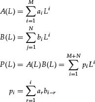
The convolution product of two infinite series in the lag operator is defined in a similar way

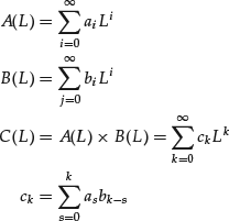
We can define the left-inverse (right-inverse) of an infinite series as the operator A−1 (L), such that A−1 (L) × A(L) = I. The inverse can always be computed solving an infinite set of recursive equations provided that a0 ≠ 0. However, the inverse series will not necessarily be stationary. A sufficient condition for stationarity is that the coefficients of the inverse series are absolutely summable.

In general, it is possible to perform on the symbolic series

the same operations that can be performed on the series

with z complex variable. However operations performed on a series of lag operators neither assume nor entail convergence properties. In fact, one can think of z simply as a symbol. In particular, the inverse does not necessarily exhibit absolutely summable coefficients.

Stationary Univariate Moving Average

Using the lag operator L notation, the infinite moving-average representation can be written as follows:

Consider now the inverse series:

If the coefficients λi are absolutely summable, we can write

and the series is said to be invertible.

Multivariate Stationary Series

The concepts of infinite moving-average representation and of invertibility defined above for univariate series carry over immediately to the multivariate case. In fact, it can be demonstrated that under mild regularity conditions, any multivariate stationary causal time series admits the following infinite moving-average representation:

where the Hi are n × n matrices, εt is an n-dimensional, zero-mean, white noise process with nonsingular variance-covariance matrix Ω, and m is an n-vector of constants. The coefficients Hi are called Markov coefficients. This moving-average representation is called the Wold representation. Wold representation states that any series where only the past influences the present can be represented as an infinite moving average of white noise terms. Note that, as in the univariate case, the infinite moving-average representation can be written in more general terms as a sum that extends from −∞ to +∞. However, a series of this type is not suitable for financial modeling as it is not causal (that is, the future influences the present). Therefore we consider only moving averages that extend to past terms.

Suppose that the Markov coefficients are an absolutely summable series:

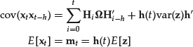
where ||H||2 indicates the largest eigenvalue of the matrix HH′. Under this assumption, it can be demonstrated that the series is stationary and that the (time-invariant) first two moments can be computed in the following way:

with the convention Hi = 0 if i < 0. Note that the assumption that the Markov coefficients are an absolutely summable series is essential, otherwise the covariance matrix would not exist. For instance, if the Hi were identity matrices, the variances of the series would become infinite.

As the second moments are all constants, the series is weakly stationary. We can write the time-independent autocovariance function of the series, which is an n × n matrix whose entries are a function of the lag h, as

Under the assumption that the Markov coefficients are an absolutely summable series, we can use the lag-operator L representation and write the operator

so that the Wold representation of a series can be written as

The concept of invertibility carries over to the multivariate case. A multivariate stationary time series is said to be invertible if it can be represented in autoregressive form. Invertibility means that the white noise process can be recovered as a function of the series. In order to explain the notion of invertible processes, it is useful to introduce the generating function of the operator H, defined as the following matrix power series:

It can be demonstrated that, if H0 = I, then H(0) = H0 and the power series H(z) is invertible in the sense that it is possible to formally derive the inverse series,

such that

where the product is intended as a convolution product. If the coefficients i are absolutely summable, as the process xt is assumed to be stationary, it can be represented in infinite autoregressive form:

In this case the process xt is said to be invertible.

From the above, it is clear that the infinite moving average representation is a more general linear representation of a stationary time than the infinite autoregressive form. A process that admits both representations is called invertible.

Nonstationary Series

Let’s now look at nonstationary series. As there is no very general model of nonstationary time series valid for all nonstationary series, we have to restrict somehow the family of admissible models. Let’s consider a family of linear, moving-average, nonstationary models of the following type:

where the Hi are left unrestricted and do not necessarily form an absolutely summable series, h(t) is deterministic, and z−1 is a random vector called the initial conditions, which is supposed to be uncorrelated with the white noise process. The essential differences of this linear model with respect to the Wold representation of stationary series are:

• The presence of a starting point and of initial conditions.
• The absence of restrictions on the coefficients.
• The index t, which restricts the number of summands.

The first two moments of a linear process are not constant. They can be computed in a way similar to the infinite moving average case:

Let’s now see how a linear process can be expressed in autoregressive form. To simplify notation let’s introduce the processes and and the deterministic series defined as follows:

It can be demonstrated that, due to the initial conditions, a linear process always satisfies the following autoregressive equation:

A random walk model

is an example of a linear nonstationary model.

The above linear model can also represent processes that are nearly stationary in the sense that they start from initial conditions but then converge to a stationary process. A process that converges to a stationary process is called asymptotically stationary.

We can summarize the previous discussion as follows. Under mild regularity conditions, any causal stationary series can be represented as an infinite moving average of a white noise process. If the series can also be represented in an autoregressive form, then the series is said to be invertible. Nonstationary series do not have corresponding general representations. Linear models are a broad class of nonstationary models and of asymptotically stationary models that provide the theoretical base for ARMA and state-space processes that will be discussed in the following sections.

ARMA REPRESENTATIONS

The infinite moving average or autoregressive representations of the previous section are useful theoretical tools but they cannot be applied to estimate processes. One needs a parsimonious representation with a finite number of coefficients. Autoregressive moving average (ARMA) models and state-space models provide such representation; though apparently conceptually different, they are statistically equivalent.

Stationary Univariate ARMA Models

Let’s start with univariate stationary processes. An autoregressive process of order p − AR(p) is a process of the form:

which can be written using the lag operator as

Not all processes that can be written in autoregressive form are stationary. In order to study the stationarity of an autoregressive process, consider the following polynomial:

where z is a complex variable.

The equation

is called the inverse characteristic equation. It can be demonstrated that if the roots of this equation, that is, its solutions, are all strictly greater than 1 in modulus (that is, the roots are outside the unit circle), then the operator A(L) is invertible and admits the inverse representation:

In order to avoid possible confusion, note that the solutions of the inverse characteristic equation are the reciprocal of the solution of the characteristic equation defined as

Therefore an autoregressive process is invertible with an infinite moving average representation that only involves positive powers of the operator L if the solutions of the characteristic equation are all strictly smaller than 1 in absolute value. This is the condition of invertibility often stated in the literature.

Let’s now consider finite moving-average representations. A process is called a moving average process of order q − MA(q) if it admits the following representation:

In a way similar to the autoregressive case, if the roots of the equation

are all strictly greater than 1 in modulus, then the MA(q) process is invertible and, therefore, admits the infinite autoregressive representation:

As in the previous case, if one considers the characteristic equation,

then the MA(q) process admits a causal autoregressive representation if the roots of the characteristic equation are strictly smaller than 1 in modulus.

Let’s now consider, more in general, an ARMA process of order p,q. We say that a stationary process admits a minimal ARMA(p, q) representation if it can be written as

or equivalently in terms of the lag operator

where εt is a serially uncorrelated white noise with nonzero variance, a0 = b0 = 1, ap ≠ 0, bq ≠ 0, the polynomials A and B have roots strictly greater than 1 in modulus and do not have any root in common.

Generalizing the reasoning in the pure MA or AR case, it can be demonstrated that a generic process that admits the ARMA(p,q) representation A(L)xt = B(L)εt is stationary if both polynomials A and B have roots strictly different from 1. In addition, if all the roots of the polynomial A(z) are strictly greater than 1 in modulus, then the ARMA(p,q) process can be expressed as a moving average process:

Conversely, if all the roots of the polynomial B(z) are strictly greater than 1, then the ARMA(p,q) process can be expressed as an autoregressive process:

Note that in the above discussions every process was centered—that is, it had zero constant mean. As we were considering stationary processes, this condition is not restrictive as the eventual nonzero mean can be subtracted.

Note also that ARMA stationary processes extend through the entire time axis. An ARMA process, which begins from some initial conditions at starting time t = 0, is not stationary even if its roots are strictly outside the unit circle. It can be demonstrated, however, that such a process is asymptotically stationary.

Nonstationary Univariate ARMA Models

So far we have considered only stationary processes. However, ARMA equations can also represent nonstationary processes if some of the roots of the polynomial A(z) are equal to 1 in modulus. A process defined by the equation

is called an autoregressive integrated moving-average (ARIMA) process if at least one of the roots of the polynomial A is equal to 1 in modulus. Suppose that λ be a root with multiplicity d. In this case the ARMA representation can be written as

However this formulation is not satisfactory as the process A is not invertible if initial conditions are not provided; it is therefore preferable to offer a more rigorous definition, which includes initial conditions. Therefore, we give the following definition of nonstationary integrated ARMA processes.

A process xt defined for t ≥ 0 is called an autoregressive integrated moving-average process—ARIMA(p,d,q)—if it satisfies a relationship of the type

where:

• The polynomials A(L) and B(L) have roots strictly greater than 1.
• εt is a white noise process defined for t ≥ 0.
• A set of initial conditions (x−1, … , x−p−d, εt, … , ε−q) independent from the white noise is given.

Later in this entry we discuss the interpretation and further properties of the ARIMA condition.

Stationary Multivariate ARMA Models

Let’s now move on to consider stationary multivariate processes. A stationary process that admits an infinite moving-average representation of the type

where εt−i is an n-dimensional, zero-mean, white-noise process with nonsingular variance-covariance matrix is called an autoregressive moving-average—ARMA(p,q)—model, if it satisfies a difference equation of the type

where A and B are matrix polynomials in the lag operator L of order p and q respectively:

If q = 0, the process is purely autoregressive of order p; if q = 0, the process is purely a moving average of order q. Rearranging the terms of the difference equation, it is clear that an ARMA process is a process where the i-th component of the process at time t, xi,t is a linear function of all the components at different lags plus a finite moving average of white noise terms.

It can be demonstrated that the ARMA representation is not unique. The nonuniqueness of the ARMA representation is due to different reasons, such as the existence of a common polynomial factor in the autoregressive and the moving-average part. It entails that the same process can be represented by models with different pairs p,q. For this reason, one would need to determine at least a minimal representation— that is, an ARMA(p,q) representation such that any other ARMA(p′,q′) representation would have p′ > p, q′ > q. With the exception of the univariate case, these problems are very difficult from a mathematical point of view and we will not examine them in detail.

Let’s now explore what restrictions on the polynomials A(L) and B(L) ensure that the relative ARMA process is stationary. Generalizing the univariate case, the mathematical analysis of stationarity is based on the analysis of the polynomial det[A(z)] obtained by formally replacing the lag operator L with a complex variable z in the matrix A(L) whose entries are finite polynomials in L.

It can be demonstrated that if the complex roots of the polynomial det[A(z)], that is, the solutions of the algebraic equation det[A(z)] = 0, which are in general complex numbers, all lie outside the unit circle, that is, their modulus is strictly greater than one, then the process that satisfies the ARMA conditions,

is stationary. As in the univariate case, if one would consider the equations in 1/z, the same reasoning applies but with roots strictly inside the unit circle.

A stationary ARMA(p,q) process is an autocorrelated process. Its time-independent autocorrelation function satisfies a set of linear difference equations. Consider an ARMA(p,q) process that satisfies the following equation:

where A0 = I. By expanding the expression for the autocovariance function, it can be demonstrated that the autocovariance function satisfies the following set of linear difference equations:

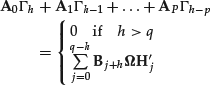
where and Hi are, respectively, the covariance matrix and the Markov coefficients of the process in its infinite moving-average representation:

From the above representation, it is clear that if the process is purely MA, that is, if p = 0, then the autocovariance function vanishes for lag h > q.

It is also possible to demonstrate the converse of this theorem. If a linear stationary process admits an autocovariance function that satisfies the following equations,

then the process admits an ARMA(p,q) representation. In particular, a stationary process is a purely finite moving-average process MA(q), if and only if its autocovariance functions vanish for h > q, where q is an integer.

Nonstationary Multivariate ARMA Models

Let’s now consider nonstationary series. Consider a series defined for t ≥ 0 that satisfies the following set of difference equations:

where, as in the stationary case, εt−i is an n-dimensional zero-mean, white noise process with nonsingular variance-covariance matrix , A0 = I, B0 = I, Ap ≠ 0, Bq ≠ 0. Suppose, in addition, that initial conditions (x−1, … ,x–p, εt, … ,ε−q) are given. Under these conditions, we say that the process xt, which is well defined, admits an ARMA representation.

A process xt is said to admit an ARIMA representation if, in addition to the above, it satisfies the following two conditions: (1) det[B(z)] has all its roots strictly outside of the unit circle, and (2) det[A(z)] has all its roots outside the unit circle but with at least one root equal to 1. In other words, an ARIMA process is an ARMA process that satisfies some additional conditions. Later in this entry we will clarify the meaning of integrated processes.

Markov Coefficients and ARMA Models

For the theoretical analysis of ARMA processes, it is useful to state what conditions on the Markov coefficients ensure that the process admits an ARMA representation. Consider a process xt, stationary or not, which admits a moving-average representation either as

or as a linear model:

The process xi admits an ARMA representation if and only if there is an integer q and a set of p matrices Ai, i = 0, … , p such that the Markov coefficients Hi satisfy the following linear difference equation starting from q:

Therefore, any ARMA process admits an infinite moving-average representation whose Markov coefficients satisfy a linear difference equation starting from a certain point. Conversely, any such linear infinite moving-average representation can be expressed parsimoniously in terms of an ARMA process.

Hankel Matrices and ARMA Models

For the theoretical analysis of ARMA processes it is also useful to restate the above conditions in terms of the Hankel infinite matrices. (A Hankel matrix is a matrix where for each antidiagonal the element is the same.) It can be demonstrated that a process, stationary or not, which admits either the infinite moving average representation

or a linear moving average model

also admits an ARMA representation if and only if the Hankel matrix formed with the sequence of its Markov coefficients has finite rank or, equivalently, a finite column rank or row rank.

INTEGRATED SERIES AND TRENDS

This section introduces the fundamental notions of trend stationary series, difference stationary series, and integrated series. Consider a one-dimensional time series. A trend stationary series is a series formed by a deterministic trend plus a stationary process. It can be written as

A trend stationary process can be transformed into a stationary process by subtracting the trend. Removing the deterministic trend entails that the deterministic trend is known. A trend stationary series is an example of an adjustment model.

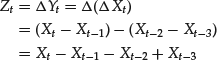
Consider now a time series Xt. The operation of differencing a series consists of forming a new series Yt = ΔXt = Xt − Xt−1. The operation of differencing can be repeated an arbitrary number of times. For instance, differencing twice the series Xt yields the following series:

Differencing can be written in terms of the lag operator as

A difference stationary series is a series that is transformed into a stationary series by differencing. A difference stationary series can be written as

where ε(t) is a zero-mean stationary process and μ is a constant. A trend stationary series with a linear trend is also difference stationary, if spac-ings are regular. The opposite is not generally true. A time series is said to be integrated of order n if it can be transformed into a stationary series by differencing n times.

Note that the concept of integrated series as defined above entails that a series extends on the entire time axis. If a series starts from a set of initial conditions, the difference sequence can only be asymptotically stationary.

There are a number of obvious differences between trend stationary and difference stationary series. A trend stationary series experiences stationary fluctuation, with constant variance, around an arbitrary trend. A difference stationary series meanders arbitrarily far from a linear trend, producing fluctuations of growing variance. The simplest example of difference stationary series is the random walk.

An integrated series is characterized by a stochastic trend. In fact, a difference stationary series can be written as

The difference Xt - Xt* between the value of a process at time t and the best affine prediction at time t − 1 is called the innovation of the process. In the above linear equation, the stationary process ε(t) is the innovation process. A key aspect of integrated processes is that innovations ε(t) never decay but keep on accumulating. In a trend stationary process, on the other hand, past innovations disappear at every new step.

These considerations carry over immediately in a multidimensional environment. Multidimensional trend stationary series will exhibit multiple trends, in principle one for each component. Multidimensional difference-stationary series will yield a stationary process after differencing.

Let’s now see how these concepts fit into the ARMA framework, starting with univariate ARMA model. Recall that an ARIMA process is defined as an ARMA process in which the polynomial B has all roots outside the unit circle while the polynomial A has one or more roots equal to 1. In the latter case the process can be written as

and we say that the process is integrated of order n. If initial conditions are supplied, the process can be inverted and the difference sequence is asymptotically stationary.

The notion of integrated processes carries over naturally in the multivariate case but with a subtle difference. Recall from earlier discussion in this entry that an ARIMA model is an ARMA model:

which satisfies two additional conditions: (1) det[B(z)] has all its roots strictly outside of the unit circle, and (2) det[A(z)] has all its roots outside the unit circle but with at least one root equal to 1.

Now suppose that, after differencing d times, the multivariate series can be represented as follows:

In this case, if (1) B′(z) is of order q and det[B′(z)] has all its roots strictly outside of the unit circle and (2) A′(z) is of order p and det[A′(z)] has all its roots outside the unit circle, then the process is called ARIMA(p,d,q). Not all ARIMA models can be put in this framework as different components might have a different order of integration.

Note that in an ARIMA(p,d,q) model each component series of the multivariate model is individually integrated. A multivariate series is integrated of order d if every component series is integrated of order d.

Note also that ARIMA processes are not invertible as infinite moving averages, but as discussed, they can be inverted in terms of a generic linear moving-average model with stochastic initial conditions. In addition, the process in the d-differences is asymptotically stationary.

In both trend stationary and difference stationary processes, innovations can be serially autocorrelated. In the ARMA representations discussed in the previous section, innovations are serially uncorrelated white noise as all the autocorrelations are assumed to be modeled in the ARMA model. If there is residual autocorrelation, the ARMA or ARIMA model is somehow misspecified.

The notion of an integrated process is essentially linear. A process is integrated if stationary innovations keep on adding indefinitely. Note that innovations could, however, cumulate in ways other than addition, producing essentially nonlinear processes. In ARCH and GARCH processes for instance, innovations do not simply add to past innovations.

The behavior of integrated and nonintegrated time series is quite different and the estimation procedures are different as well. It is therefore important to ascertain if a series is integrated or not. Often a preliminary analysis to ascertain integratedness suggests what type of model should be used.

A number of statistical tests to ascertain if a univariate series is integrated are available. Perhaps the most widely used and known are the Dickey-Fuller (DF) and the Augmented Dickey-Fuller (ADF) tests. The DF test assumes as a null hypothesis that the series is integrated of order 1 with uncorrelated innovations. Under this assumption, the series can be written as a random walk in the following form:

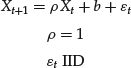
where IID is an independent and identical sequence.

In a sample generated by a model of this type, the value of ρ estimated on the sample is stochastic. Estimation can be performed with the ordinary least square (OLS) method. Dickey and Fuller determined the theoretical distribution of ρ and computed the critical values of ρ that correspond to different confidence intervals. The theoretical distribution of ρ is determined computing a functional of the Brownian motion.

Given a sample of a series, for instance a series of log prices, application of the DF test entails computing the autoregressive parameter ρ on the given sample and comparing it with the known critical values for different confidence intervals. The strict hypothesis of random walk is too strong for most econometric applications. The DF test was extended to cover the case of correlated residuals that are modeled as a linear model. In the latter case, the DF test is called the Augmented Dickey-Fuller or ADF test. The Phillips and Perron test is the DF test in the general case of autocorrelated residuals.

APPENDIX

We will begin with several concepts from probability theory.

Stochastic Processes

When it is necessary to emphasize the dependence of the random variable from both time t and the element ω, a stochastic process is explicitly written as a function of two variables: X = X(t,ω). Given ω, the function X = Xt(ω) is a function of time that is referred to as the path of the stochastic process.

The variable X might be a single random variable or a multidimensional random vector. A stochastic process is therefore a function X = X(t, ω) from the product space [0,T] × Ω into the n-dimensional real space Rn. Because to each co corresponds a time path of the process—in general formed by a set of functions X = Xt(ω)—it is possible to identify the space Ω with a subset of the real functions defined over an interval [0,T].

Let’s now discuss how to represent a stochastic process X = X(t,ω) and the conditions of identity of two stochastic processes. As a stochastic process is a function of two variables, we can define equality as pointwise identity for each couple (t, ω). However, as processes are defined over probability spaces, pointwise identity is seldom used. It is more fruitful to define equality modulo sets of measure zero or equality with respect to probability distributions. In general, two random variables X,Y will be considered equal if the equality X(ω) = Y(ω) holds for every ω with the exception of a set of probability zero. In this case, it is said that the equality holds almost everywhere (denoted a.e.).

A rather general (but not complete) representation is given by the finite dimensional probability distributions. Given any set of indices t1, … , tm, consider the distributions

These probability measures are, for any choice of the ti, the finite-dimensional joint probabilities of the process. They determine many, but not all, properties of a stochastic process. For example, the finite dimensional distributions of a Brownian motion do not determine whether or not the process paths are continuous.

In general, the various concepts of equality between stochastic processes can be described as follows:

• Property 1. Two stochastic processes are weakly equivalent if they have the same finite-dimensional distributions. This is the weakest form of equality.
• Property 2. The process X = X(t,ω) is said to be equivalent or to be a modification of the process Y = Y(t,ω) if, for all t,

  

• Property 3. The process X = X(t, ω) is said to be strongly equivalent to or indistinguishable from the process Y = Y(t, ω) if

  

Property 3 implies Property 2, which in turn implies Property 1. Implications do not hold in the opposite direction. Two processes having the same finite distributions might have completely different paths. However it is possible to demonstrate that if one assumes that paths are continuous functions of time, Properties 2 and 3 become equivalent.

Information Structures

Let’s now turn our attention to the question of time. We must introduce an appropriate representation of time as well as rules that describe the evolution of information, that is, information propagation, over time. The concepts of information and information propagation are fundamental in economics and finance theory.

The concept of information in finance is different from both the intuitive notion of information and that of information theory in which information is a quantitative measure related to the a priori probability of messages. In our context, information means the (progressive) revelation of the set of events to which the current state of the economy belongs. Though somewhat technical, this concept of information sheds light on the probabilistic structure of finance theory. The point is the following. Assets are represented by stochastic processes, that is, time-dependent random variables. But the probabilistic states on which these random variables are defined represent entire histories of the economy. To embed time into the probabilistic structure of states in a coherent way calls for information structures and filtrations (a concept we explain next).

It is assumed that the economy is in one of many possible states and that there is uncertainty on the state that has been realized. Consider a time period of the economy. At the beginning of the period, there is complete uncertainty on the state of the economy (i.e., there is complete uncertainty on what path the economy will take). Different events have different probabilities, but there is no certainty. As time passes, uncertainty is reduced as the number of states to which the economy can belong is progressively reduced. Intuitively, revelation of information means the progressive reduction of the number of possible states; at the end of the period, the realized state is fully revealed. In continuous time and continuous states, the number of events is infinite at each instant. Thus its cardinality remains the same. We cannot properly say that the number of events shrinks. A more formal definition is required.

The progressive reduction of the set of possible states is formally expressed in the concepts of information structure and filtration. Let’s start with information structures. Information structures apply only to discrete probabilities defined over a discrete set of states. At the initial instant T0, there is complete uncertainty on the state of the economy; the actual state is known only to belong to the largest possible event (that is, the entire space Ω). At the following instant T1, assuming that instants are discrete, the states are separated into a partition, a partition being a denumerable class of disjoint sets whose union is the space itself. The actual state belongs to one of the sets of the partitions. The revelation of information consists in ruling out all sets but one. For all the states of each partition, and only for these, random variables assume the same values.

Suppose, to exemplify, that only two assets exist in the economy and that each can assume only two possible prices and pay only two possible cash flows. At every moment there are 16 possible price-cash flow combinations. We can thus see that at the moment T1 all the states are partitioned into 16 sets, each containing only one state. Each partition includes all the states that have a given set of prices and cash distributions at the moment T1. The same reasoning can be applied to each instant. The evolution of information can thus be represented by a tree structure in which every path represents a state and every point a partition. Obviously the tree structure does not have to develop as symmetrically as in the above example; the tree might have a very generic structure of branches.

Filtration

The concept of information structure based on partitions provides a rather intuitive representation of the propagation of information through a tree of progressively finer partitions. However, this structure is not sufficient to describe the propagation of information in a general probabilistic context. In fact, the set of possible events is much richer than the set of partitions. It is therefore necessary to identify not only partitions but also a structure of events. The structure of events used to define the propagation of information is called a filtration. In the discrete case, however, the two concepts—information structure and filtration—are equivalent.

The concept of filtration is based on identifying all events that are known at any given instant. It is assumed that it is possible to associate to each trading moment t a σ-algebra of events t ⊂ formed by all events that are known prior to or at time t. It is assumed that events are never “forgotten,” that is, that t ⊂ S, if t < s. An ordering of time is thus created. This ordering is formed by an increasing sequence of σ-algebras, each associated to the time at which all its events are known. This sequence is a filtration. Indicated as {t}, a filtration is therefore an increasing sequence of all σ-algebras t, each associated to an instant t.

In the finite case, it is possible to create a mutual correspondence between filtrations and information structures. In fact, given an information structure, it is possible to associate to each partition the algebra generated by the same partition. Observe that a tree information structure is formed by partitions that create increasing refinement: By going from one instant to the next, every set of the partition is decomposed. One can then conclude that the algebras generated by an information structure form a filtration.

On the other hand, given a filtration {t}, it is possible to associate a partition to each t. In fact, given any element that belongs to Ω, consider any other element that belongs to Ω such that, for each set of t, both either belong to or are outside this set. It is easy to see that classes of equivalence are thus formed, that these create a partition, and that the algebra generated by each such partition is precisely the t that has generated the partition.

A stochastic process is said to be adapted to the filtration {t} if the variable Xt is measurable with respect to the σ-algebra t. It is assumed that the price and cash distribution processes St(ω) and dt(ω) of every asset are adapted to {t}. This means that, for each t, no measurement of any price or cash distribution variable can identify events not included in the respective algebra or σ-algebra. Every random variable is a partial image of the set of states seen from a given point of view and at a given moment.

The concepts of filtration and of processes adapted to a filtration are fundamental. They ensure that information is revealed without anticipation. Consider the economy and associate at every instant a partition and an algebra generated by the partition. Every random variable defined at that moment assumes a value constant on each set of the partition. The knowledge of the realized values of the random variables does not allow identifying sets of events finer than partitions.

One might well ask: Why introduce the complex structure of σ-algebras as opposed to simply defining random variables? The point is that, from a logical point of view, the primitive concept is that of states and events. The evolution of time has to be defined on the primitive structure—it cannot simply be imposed on random variables. In practice, filtrations become an important concept when dealing with conditional probabilities in a continuous environment. As the probability that a continuous random variable assumes a specific value is zero, the definition of conditional probabilities requires the machinery of filtration.

Conditional Probability and Conditional Expectation

Conditional probabilities and conditional averages are fundamental in the stochastic description of financial markets. For instance, one is generally interested in the probability distribution of the price of an asset at some date given its price at an earlier date. The widely used regression models are an example of conditional expectation models.

The conditional probability of event A given event B was defined earlier as

This simple definition cannot be used in the context of continuous random variables because the conditioning event (i.e., one variable assuming a given value) has probability zero. To avoid this problem, we condition on σ-algebras and not on single zero-probability events. In general, as each instant is characterized by a σ-algebra t, the conditioning elements are the t.

The general definition of conditional expectation is the following. Consider a probability space (Ω, , P) and a σ-algebra contained in and suppose that X is an integrable random variable on (Ω, , P). We define the conditional expectation of X with respect to , written as E[X|], as a random variable measurable with respect to such that

for every set G . In other words, the conditional expectation is a random variable whose average on every event that belongs to is equal to the average of X over those same events, but it is -measurable while X is not. It is possible to demonstrate that such variables exist and are unique up to a set of measure zero.

Econometric models usually condition a random variable given another variable. In the previous framework, conditioning one random variable X with respect to another random variable Y means conditioning X given σ{Y} (i.e., given the σ-algebra generated by Y). Thus E[X|Y] means E[X|σ{Y}].

This notion might seem to be abstract and to miss a key aspect of conditioning: intuitively, conditional expectation is a function of the conditioning variable. For example, given a stochastic price process, Xt, one would like to visualize conditional expectation E[Xt | Xs], s < t as a function of Xs that yields the expected price at a future date given the present price. This intuition is not wrong insofar as the conditional expectation E[X| Y] of X given Y is a random variable function of Y.

However, we need to specify how conditional expectations are formed, given that the usual conditional probabilities cannot be applied as the conditioning event has probability zero. Here is where the above definition comes into play. The conditional expectation of a variable X given a variable Y is defined in full generality as a variable that is measurable with respect to the σ-algebra σ(Y) generated by the conditioning variable Y and has the same expected value of Y on each set of σ(Y). Later in this section we will see how conditional expectations can be expressed in terms of the joint p.d.f. of the conditioning and conditioned variables.

One can define conditional probabilities starting from the concept of conditional expectations. Consider a probability space (Ω, , P), a sub-σ-algebra of , and two events A , B . If IA,IB are the indicator functions of the sets A,B (the indicator function of a set assumes value 1 on the set, 0 elsewhere), we can define conditional probabilities of the event A, respectively, given or given the event B as

Using these definitions, it is possible to demonstrate that given two random variables X and Y with joint density f(x, y), the conditional density of X given Y is

where the marginal density, defined as

is assumed to be strictly positive.

In the discrete case, the conditional expectation is a random variable that takes a constant value over the sets of the finite partition associated to t. Its value for each element of Ω is defined by the classical concept of conditional probability. Conditional expectation is simply the average over a partition assuming the classical conditional probabilities.

An important econometric concept related to conditional expectations is that of a martingale. Given a probability space (,,P) and a filtration {t}, a sequence of i-measurable random variables Xi is called a martingale if the following condition holds:

A martingale translates the idea of a “fair game” as the expected value of the variable at the next period is the present value of the same value.

KEY POINTS

• Stochastic processes are time-dependent random variables.
• An information structure is a collection of partitions of events associated to each instant of time that become progressively finer with the evolution of time. A filtration is an increasing collection of σ-algebras associated to each instant of time.
• The states of the economy, intended as full histories of the economy, are represented as a probability space.  The revelation of information with time is represented by information structures or filtrations. Prices and other financial quantities are represented by adapted stochastic processes.
• By conditioning is meant the change in probabilities due to the acquisition of some information. It is possible to condition with respect to an event if the event has nonzero probability. In general terms, conditioning means conditioning with respect to a filtration or an information structure.
• A martingale is a stochastic process such that the conditional expected value is always equal to its present value. It embodies the idea of a fair game where today’s wealth is the best forecast of future wealth.
• A time series is a discrete-time stochastic process, that is, a denumerable collection of random variables indexed by integer numbers.
• Any stationary time series admits an infinite moving average representation, that is to say, it can be represented as an infinite sum of white noise terms with appropriate coefficients.
• A time series is said to be invertible if it can also be represented as an infinite autoregression, that is, an infinite sum of all past terms with appropriate coefficients.
• ARMA models are parsimonious representations that involve only a finite number of moving average and autoregressive terms.
• An ARMA model is stationary if all the roots of the inverse characteristic equation of the AR or the MA part have roots with modulus strictly greater than one.
• A process is said to be integrated of order p if it becomes stationary after differencing p times.

NOTE

1. See Enders (2009), Gourieroux and Monfort (1997), Hamilton (1994), and Tsay (2001) for a comprehensive discussion of modern time series econometrics.

REFERENCES

Enders, W. (2009). Applied Econometric Time Series: 3rd Ed. Hoboken, NJ: John Wiley & Sons.

Gourieroux, C., and Monfort, A. (1997). Time Series and Dynamic Models. Cambridge: Cambridge University Press.

Hamilton, J. D. (1994). Time Series Analysis. Princeton, NJ: Princeton University Press.

Tsay, R.S. (2001). Analysis of Financial Time Series. Hoboken, NJ: John Wiley & Sons.