ARCH/GARCH Models in Applied Financial Econometrics

ROBERT F. ENGLE, PhD

Michael Armellino Professorship in the Management of Financial Services and Director of the Volatility Institute, Leonard N. Stern School of Business, New York University

SERGIO M. FOCARDI, PhD

Partner, The Intertek Group

FRANK J. FABOZZI, PhD, CFA, CPA

Professor of Finance, EDHEC Business School

In this entry we discuss the modeling of the time behavior of the uncertainty related to many econometric models when applied to financial data. Finance practitioners know that errors made in predicting markets are not of a constant magnitude. There are periods when unpredictable market fluctuations are larger and periods when they are smaller. This behavior, known as heteroskedasticity, refers to the fact that the size of market volatility tends to cluster in periods of high volatility and periods of low volatility. The discovery that it is possible to formalize and generalize this observation was a major breakthrough in econometrics. In fact, we can describe many economic and financial data with models that predict, simultaneously, the economic variables and the average magnitude of the squared prediction error.

In this entry, we show how the average error size can be modeled as an autoregressive process. Given their autoregressive nature, these models are called autoregressive conditional heteroskedasticity (ARCH) or generalized autoregressive conditional heteroskedasticity (GARCH). This discovery is particularly important in financial econometrics, where the error size is, in itself, a variable of great interest.

REVIEW OF LINEAR REGRESSION AND AUTOREGRESSIVE MODELS

Let’s first discuss two examples of basic econometric models, the linear regression model and the autoregressive model, and illustrate the meaning of homoskedasticity or heteroskedasticity in each case.

The linear regression model is the workhorse of economic modeling. A univariate linear regression represents a proportionality relationship between two variables:

The preceding linear regression model states that the expectation of the variable y is β times the expectation of the variable x plus a constant α. The proportionality relationship between y and x is not exact but subject to an error ε.

In standard regression theory, the error ε is assumed to have a zero mean and a constant standard deviation σ. The standard deviation is the square root of the variance, which is the expectation of the squared error: . It is a positive number that measures the size of the error. We call homoskedasticity the assumption that the expected size of the error is constant and does not depend on the size of the variable x. We call heteroskedasticity the assumption that the expected size of the error term is not constant.

The assumption of homoskedasticity is convenient from a mathematical point of view and is standard in regression theory. However, it is an assumption that must be verified empirically. In many cases, especially if the range of variables is large, the assumption of homo-skedasticity might be unreasonable. For example, assuming a linear relationship between consumption and household income, we can expect that the size of the error depends on the size of household income. In fact, high-income households have more freedom in the allocation of their income.

In the preceding household-income example, the linear regression represents a cross-sectional model without any time dimension. However, in finance and economics in general, we deal primarily with time series, that is, sequences of observations at different moments of time. Let’s call Xt the value of an economic time series at time t. Since the groundbreaking work of Haavelmo (1944), economic time series are considered to be realizations of stochastic processes. That is, each point of an economic time series is considered to be an observation of a random variable.

We can look at a stochastic process as a sequence of variables characterized by joint-probability distributions for every finite set of different time points. In particular, we can consider the distribution ft of each variable Xt at each moment. Intuitively, we can visualize a stochastic process as a very large (infinite) number of paths. A process is called weakly stationary if all of its second moments are constant. In particular this means that the mean and variance are constants and that do not depend on the time t. A process is called strictly stationary if none of its finite distributions depends on time. A strictly stationary process is not necessarily weakly stationary as its finite distributions, though time-independent, might have infinite moments.

The terms and are the unconditional mean and variance of a process. In finance and economics, however, we are typically interested in making forecasts based on past and present information. Therefore, we consider the distribution of the variable at time t2 conditional on the information known at time t1. Based on information available at time t − 1, It−1, we can also define the conditional mean and the conditional variance .

A process can be weakly stationary but have time-varying conditional variance. If the conditional mean is constant, then the unconditional variance is the unconditional expectation of the conditional variance. If the conditional mean is not constant, the unconditional variance is not equal to the unconditional expectation of the conditional variance; this is due to the dynamics of the conditional mean.

In describing ARCH/GARCH behavior, we focus on the error process. In particular, we assume that the errors are an innovation process, that is, we assume that the conditional mean of the errors is zero. We write the error process as: where is the conditional standard deviation and the z terms are a sequence of independent, zero-mean, unit-variance, normally distributed variables. Under this assumption, the unconditional variance of the error process is the unconditional mean of the conditional variance. Note, however, that the unconditional variance of the process variable does not, in general, coincide with the unconditional variance of the error terms.

In financial and economic models, conditioning is often stated as regressions of the future values of the variables on the present and past values of the same variable. For example, if we assume that time is discrete, we can express conditioning as an autoregressive model:

The error term is conditional on the information Ii that, in this example, is represented by the present and the past n values of the variable X. The simplest autoregressive model is the random walk model of the logarithms of prices pi:

In terms of returns, the random walk model is simply:

A major breakthrough in econometric modeling was the discovery that, for many families of econometric models, linear and nonlinear alike, it is possible to specify a stochastic process for the error terms and predict the average size of the error terms when models are fitted to empirical data. This is the essence of ARCH modeling introduced by Engle (1982).

Two observations are in order. First, we have introduced two different types of heteroskedasticity. In the first example, regression errors are heteroskedastic because they depend on the value of the independent variables: The average error is larger when the independent variable is larger. In the second example, however, error terms are conditionally heteroskedastic because they vary with time and do not necessarily depend on the value of the process variables. Later in this entry we will describe a variant of the ARCH model where the size of volatility is correlated with the level of the variable. However, in the basic specification of ARCH models, the level of the variables and the size of volatility are independent.

Second, let’s observe that the volatility (or the variance) of the error term is a hidden, nonobservable variable. Later in this entry, we will describe realized volatility models that treat volatility as an observed variable. Theoretically, however, time-varying volatility can be only inferred, not observed. As a consequence, the error term cannot be separated from the rest of the model. This occurs both because we have only one realization of the relevant time series and because the volatility term depends on the model used to forecast expected returns. The ARCH/GARCH behavior of the error term depends on the model chosen to represent the data. We might use different models to represent data with different levels of accuracy. Each model will be characterized by a different specification of heteroskedasticity.

Consider, for example, the following model for returns:

In this simple model, the clustering of volatility is equivalent to the clustering of the squared returns (minus their constant mean). Now suppose that we discover that returns are predictable through a regression on some predictor f:

As a result of our discovery, we can expect that the model will be more accurate, the size of the errors will decrease, and the heteroskedastic behavior will change.

Note that in the model , the errors coincide with the fluctuations of returns around their unconditional mean. If errors are an innovation process, that is, if the conditional mean of the errors is zero, then the variance of returns coincides with the variance of errors, and ARCH behavior describes the fluctuations of returns. However, if we were able to make conditional forecasts of returns, then the ARCH model describes the behavior of the errors and it is no longer true that the unconditional variance of errors coincides with the unconditional variance of returns. Thus, the statement that ARCH models describe the time evolution of the variance of returns is true only if returns have a constant expectation.

ARCH/GARCH effects are important because they are very general. It has been found empirically that most model families presently in use in econometrics and financial econometrics exhibit conditionally heteroskedastic errors when applied to empirical economic and financial data. The heteroskedasticity of errors has not disappeared with the adoption of more sophisticated models of financial variables. The ARCH/GARCH specification of errors allows one to estimate models more accurately and to forecast volatility.

ARCH/GARCH MODELS

In this section, we discuss univariate ARCH and GARCH models. Because in this entry we focus on financial applications, we will use financial notation. Let the dependent variable, which might be the return on an asset or a portfolio, be labeled rt. The mean value m and the variance h will be defined relative to a past information set. Then the return r in the present will be equal to the conditional mean value of r (that is, the expected value of r based on past information) plus the conditional standard deviation of r (that is, the square root of the variance) times the error term for the present period:

The econometric challenge is to specify how the information is used to forecast the mean and variance of the return conditional on the past information. While many specifications have been considered for the mean return and used in efforts to forecast future returns, rather simple specifications have proven surprisingly successful in predicting conditional variances.

First, note that if the error terms were strict white noise (that is, zero-mean, independent variables with the same variance), the conditional variance of the error terms would be constant and equal to the unconditional variance of errors. We would be able to estimate the error variance with the empirical variance:

using the largest possible available sample. However, it was discovered that the residuals of most models used in financial econometrics exhibit a structure that includes heteroskedasticity and autocorrelation of their absolute values or of their squared values.

The simplest strategy to capture the time dependency of the variance is to use a short rolling window for estimates. In fact, before ARCH, the primary descriptive tool to capture time-varying conditional standard deviation and conditional variance was the rolling standard deviation or the rolling variance. This is the standard deviation or variance calculated using a fixed number of the most recent observations. For example, a rolling standard deviation or variance could be calculated every day using the most recent month (22 business days) of data. It is convenient to think of this formulation as the first ARCH model; it assumes that the variance of tomorrow’s return is an equally weighted average of the squared residuals of the last 22 days.

The idea behind the use of a rolling window is that the variance changes slowly over time, and it is therefore approximately constant on a short rolling-time window. However, given that the variance changes over time, the assumption of equal weights seems unattractive: It is reasonable to consider that more recent events are more relevant and should therefore have higher weights. The assumption of zero weights for observations more than one month old is also unappealing.

In the ARCH model proposed by Engle (1982), these weights are parameters to be estimated. Engle’s ARCH model thereby allows the data to determine the best weights to use in forecasting the variance. In the original formulation of the ARCH model, the variance is forecasted as a moving average of past error terms:

where the coefficients must be estimated from empirical data. The errors themselves will have the form

where the z terms are independent, standard normal variables (that is, zero-mean, unit-variance, normal variables). In order to ensure that the variance is nonnegative, the constants must be nonnegative. If , the ARCH process is weakly stationary with constant unconditional variance:

Two remarks should be made. First, ARCH is a forecasting model insofar as it forecasts the error variance at time t on the basis of information known at time t − 1. Second, forecasting is conditionally deterministic, that is, the ARCH model does not leave any uncertainty on the expectation of the squared error at time t knowing past errors. This must always be true of a forecast, but, of course, the squared error that occurs can deviate widely from this forecast value.

A useful generalization of this model is the GARCH parameterization introduced by Bollerslev (1986). This model is also a weighted average of past squared residuals, but it has declining weights that never go completely to zero. In its most general form, it is not a Markovian model, as all past errors contribute to forecast volatility. It gives parsimonious models that are easy to estimate and, even in its simplest form, has proven surprisingly successful in predicting conditional variances.

The most widely used GARCH specification asserts that the best predictor of the variance in the next period is a weighted average of the long-run average variance, the variance predicted for this period, and the new information in this period that is captured by the most recent squared residual. Such an updating rule is a simple description of adaptive or learning behavior and can be thought of as Bayesian updating. Consider the trader who knows that the long-run average daily standard deviation of the Standard and Poor’s 500 is 1%, that the forecast he made yesterday was 2%, and the unexpected return observed today is 3%. Obviously, this is a high-volatility period, and today is especially volatile, suggesting that the volatility forecast for tomorrow could be even higher. However, the fact that the long-term average is only 1% might lead the forecaster to lower his forecast. The best strategy depends on the dependence between days. If these three numbers are each squared and weighted equally, then the new forecast would be . However, rather than weighting these equally, for daily data it is generally found that weights such as those in the empirical example of (0.02, 0.9, 0.08) are much more accurate. Hence, the forecast is . To be precise, we can use ht to define the variance of the residuals of a regression . In this definition, the variance of is one. Therefore, a GARCH(1,1) model for variance looks like this:

This model forecasts the variance of date t return as a weighted average of a constant, yesterday’s forecast, and yesterday’s squared error. If we apply the previous formula recursively, we obtain an infinite weighted moving average. Note that the weighting coefficients are different from those of a standard exponentially weighted moving average (EWMA). The econometrician must estimate the constants ; updating simply requires knowing the previous forecast h and the residual.

The weights are and the long-run average variance is . It should be noted that this works only if and it really makes sense only if the weights are positive, requiring . In fact, the GARCH(1,1) process is weakly stationary if . If , the process is strictly stationary. The GARCH model with is called an integrated GARCH or IGARCH. It is a strictly stationary process with infinite variance.

The GARCH model described above and typically referred to as the GARCH(1,1) model derives its name from the fact that the 1,1 in parentheses is a standard notation in which the first number refers to the number of autoregressive lags (or ARCH terms) that appear in the equation and the second number refers to the number of moving average lags specified (often called the number of GARCH terms). Models with more than one lag are sometimes needed to find good variance forecasts. Although this model is directly set up to forecast for just one period, it turns out that, based on the one-period forecast, a two-period forecast can be made. Ultimately, by repeating this step, long-horizon forecasts can be constructed. For the GARCH(1,1), the two-step forecast is a little closer to the long-run average variance than is the one-step forecast, and, ultimately, the distant-horizon forecast is the same for all time periods as long as . This is just the unconditional variance. Thus, GARCH models are mean reverting and conditionally heteroskedastic but have a constant unconditional variance.

Let’s now address the question of how the econometrician can estimate an equation like the GARCH(1,1) when the only variable on which there are data is rt. One possibility is to use maximum likelihood by substituting ht for in the normal likelihood and then maximizing with respect to the parameters. GARCH estimation is implemented in commercially available software such as EViews, GAUSS, Matlab, RATS, SAS, or TSP. The process is quite straightforward: For any set of parameters and a starting estimate for the variance of the first observation, which is often taken to be the observed variance of the residuals, it is easy to calculate the variance forecast for the second observation. The GARCH updating formula takes the weighted average of the unconditional variance, the squared residual for the first observation, and the starting variance and estimates the variance of the second observation. This is input into the forecast of the third variance, and so forth. Eventually, an entire time series of variance forecasts is constructed.

Ideally, this series is large when the residuals are large and small when the residuals are small. The likelihood function provides a systematic way to adjust the parameters to give the best fit. Of course, it is possible that the true variance process is different from the one specified by the econometrician. In order to check this, a variety of diagnostic tests are available. The simplest is to construct the series of , which are supposed to have constant mean and variance if the model is correctly specified. Various tests, such as tests for autocorrelation in the squares, can detect model failures. The Ljung-Box test with 15 lagged autocorrelations is often used.

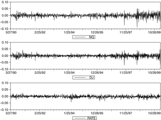
Figure 1 Nasdaq, Dow Jones, and Bond Returns

Application to Value at Risk

Applications of the ARCH/GARCH approach are widespread in situations where the volatility of returns is a central issue. Many banks and other financial institutions use the idea of value at risk (VaR) as a way to measure the risks in their portfolios.

Table 1 Portfolio Data

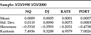
The 1% VaR is defined as the number of dollars that one can be 99% certain exceeds any losses for the next day. Let’s use the GARCH(1,1) tools to estimate the 1% VaR of a $1 million portfolio on March 23, 2000. This portfolio consists of 50% Nasdaq, 30% Dow Jones, and 20% long bonds. We chose this date because, with the fall of equity markets in the spring of 2000, it was a period of high volatility. First, we construct the hypothetical historical portfolio. (All calculations in this example were done with the EViews software program.) Figure 1 shows the pattern of the Nasdaq, Dow Jones, and long Treasury bonds. In Table 1, we present some illustrative statistics for each of these three investments separately and, in the final column, for the portfolio as a whole. Then we forecast the standard deviation of the portfolio and its 1% quantile. We carry out this calculation over several different time frames: the entire 10 years of the sample up to March 23, 2000, the year before March 23, 2000, and from January 1, 2000 to March 23, 2000.

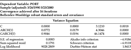
Table 2 GARCH(1,1)

Consider first the quantiles of the historical portfolio at these three different time horizons. Over the full 10-year sample, the 1% quantile times $1 million produces a VaR of $22,477. Over the last year, the calculation produces a VaR of $24,653—somewhat higher, but not significantly so. However, if the first quantile is calculated based on the data from January 1, 2000, to March 23, 2000, the VaR is $35,159. Thus, the level of risk has increased significantly over the last quarter.

The basic GARCH(1,1) results are given in Table 2. Notice that the coefficients sum up to a number slightly less than one. The forecasted standard deviation for the next day is 0.014605, which is almost double the average standard deviation of 0.0083 presented in the last column of Table 1. If the residuals were normally distributed, then this would be multiplied by 2.326348, giving a VaR equal to $33,977. As it turns out, the standardized residuals, which are the estimated values of , have a 1% quantile of 2.8437, which is well above the normal quantile. The estimated 1% VaR is $39,996. Notice that this VaR has risen to reflect the increased risk in 2000.

Finally, the VaR can be computed based solely on estimation of the quantile of the forecast distribution. This has been proposed by Engle and Manganelli (2001), adapting the quantile regression methods of Koenker and Basset (1978). Application of their method to this dataset delivers a VaR of $38,228. Instead of assuming the distribution of return series, Engle and Manganelli (2004) propose a new VaR modeling approach, conditional autoregressive value at risk (CAViaR), to directly compute the quantile of an individual financial asset. On a theoretical level, due to structural changes of the return series, the constant-parameter CAViaR model can be extended. Huang et al. (2010) formulate a time-varying CAViaR model, which they call an index-exciting time-varying CAViaR model. The model incorporates the market index information to deal with the unobservable structural break points for the individual risky asset.

WHY ARCH/GARCH?

The ARCH/GARCH framework proved to be very successful in predicting volatility changes. Empirically, a wide range of financial and economic phenomena exhibit the clustering of volatilities. As we have seen, ARCH/GARCH models describe the time evolution of the average size of squared errors, that is, the evolution of the magnitude of uncertainty. Despite the empirical success of ARCH/GARCH models, there is no real consensus on the economic reasons why uncertainty tends to cluster. That is why models tend to perform better in some periods and worse in other periods.

It is relatively easy to induce ARCH behavior in simulated systems by making appropriate assumptions on agent behavior. For example, one can reproduce ARCH behavior in artificial markets with simple assumptions on agent decision-making processes. The real economic challenge, however, is to explain ARCH/GARCH behavior in terms of features of agents behavior and/or economic variables that could be empirically ascertained.

In classical physics, the amount of uncertainty inherent in models and predictions can be made arbitrarily low by increasing the precision of initial data. This view, however, has been challenged in at least two ways. First, quantum mechanics has introduced the notion that there is a fundamental uncertainty in any measurement process. The amount of uncertainty is prescribed by the theory at a fundamental level. Second, the theory of complex systems has shown that nonlinear complex systems are so sensitive to changes in initial conditions that, in practice, there are limits to the accuracy of any model. ARCH/GARCH models describe the time evolution of uncertainty in a complex system.

In financial and economic models, the future is always uncertain but over time we learn new information that helps us forecast this future. As asset prices reflect our best forecasts of the future profitability of companies and countries, these change whenever there is news. ARCH/GARCH models can be interpreted as measuring the intensity of the news process. Volatility clustering is most easily understood as news clustering. Of course, many things influence the arrival process of news and its impact on prices. Trades convey news to the market and the macroeconomy can moderate the importance of the news. These can all be thought of as important determinants of the volatility that is picked up by ARCH/GARCH.

GENERALIZATIONS OF THE ARCH/GARCH MODELS

Thus far, we have described the fundamental ARCH and GARCH models and their application to VaR calculations. The ARCH/GARCH framework proved to be a rich framework and many different extensions and generalizations of the initial ARCH/GARCH models have been proposed. We will now describe some of these generalizations and extensions. We will focus on applications in finance and will continue to use financial notation assuming that our variables represent returns of assets or of portfolios.

Let’s first discuss why we need to generalize the ARCH/GARCH models. There are three major extensions and generalizations:

Integration of First, Second, and Higher Moments

In the ARCH/GARCH models considered thus far, returns are assumed to be normally distributed and the forecasts of the first and second moments independent. These assumptions can be generalized in different ways, either allowing the conditional distribution of the error terms to be non-normal and/or integrating the first and second moments.

Let’s first consider asymmetries in volatility forecasts. There is convincing evidence that the direction does affect volatility. Particularly for broad-based equity indexes and bond market indexes, it appears that market declines forecast higher volatility than do comparable market increases. There are now a variety of asymmetric GARCH models, including the exponential GARCH (EGARCH) model of Nelson (1991), the threshold ARCH (TARCH) model attributed to Rabemananjara and Zakoian (1993) and Glosten, Jagannathan, and Runkle (1993), and a collection and comparison by Engle and Ng (1993).

In order to illustrate asymmetric GARCH, consider, for example, the asymmetric GARCH(1,1) model of Glosten, Jagannathan, and Runkle (1993). In this model, we add a term to the basic GARCH:

The term is an indicator function that is zero when the error is positive and 1 when it is negative. If is positive, negative errors are leveraged. The parameters of the model are assumed to be positive. The relationship is assumed to hold.

In addition to asymmetries, it has been empirically found that residuals of ARCH/GARCH models fitted to empirical financial data exhibit excess kurtosis. One way to handle this problem is to consider non-normal distributions of errors. Non-normal distributions of errors were considered by Bollerslev (1987), who introduced a GARCH model where the variable z follows a Student-t distribution.

Let’s now discuss the integration of first and second moments through the GARCH-M model. ARCH/GARCH models imply that the risk inherent in financial markets varies over time. Given that financial markets implement a risk-return trade-off, it is reasonable to ask whether changing risk entails changing returns. Note that, in principle, predictability of returns in function of predictability of risk is not a violation of market efficiency. To correlate changes in volatility with changes in returns, Engle, Lilien, and Robins (1987) proposed the GARCH-M model (not to be confused with the multivariate MGARCH model that will be described shortly). The GARCH-M model, or GARCH in mean model, is a complete nonlinear model of asset returns and not only a specification of the error behavior. In the GARCH-M model, returns are assumed to be a constant plus a term proportional to the conditional variance:

where follows a GARCH process and the z terms are independent and identically distributed (IID) normal variables. Alternatively, the GARCH-M process can be specified making the mean linear in the standard deviation but not in the variance.

The integration of volatilities and expected returns, that is the integration of risk and returns, is a difficult task. The reason is that not only volatilities but also correlations should play a role. The GARCH-M model was extended by Bollerslev (1986) in a multivariate context. The key challenge of these extensions is the explosion in the number of parameters to estimate; we will see this when discussing multivariate extensions in the following sections.

Generalizations to High-Frequency Data

With the advent of electronic trading, a growing amount of data has become available to practitioners and researchers. In many markets, data at transaction level, called tick-by-tick data or ultra-high-frequency data, are now available. The increase of data points in moving from daily data to transaction data is significant. For example, the average number of daily transactions for U.S. stocks in the Russell 1000 is in the order of 2,000. Thus, we have a 2,000-fold increase in data going from daily data to tick-by-tick data.

The interest in high-frequency data is twofold. First, researchers and practitioners want to find events of interest. For example, the measurement of intraday risk and the discovery of trading profit opportunities at short time horizons are of interest to many financial institutions. Second, researchers and practitioners would like to exploit high-frequency data to obtain more precise forecasts at the usual forecasting horizon. Let’s focus on the latter objective.

As observed by Merton (1980), while in diffusive processes the estimation of trends requires long stretches of data, the estimation of volatility can be done with arbitrary precision using data extracted from arbitrarily short time periods provided that the sampling rate is arbitrarily high. In other words, in diffusive models, the estimation of volatility greatly profits from high-frequency data. It therefore seems tempting to use data at the highest possible frequency, for example spaced at a few minutes, to obtain better estimates of volatility at the frequency of practical interest, say daily or weekly. As we will see, the question is not so straightforward and the answer is still being researched.

We will now give a brief account of the main modeling strategies and the main obstacles in using high-frequency data for volatility estimates. We will first assume that the return series are sampled at a high but fixed frequency. In other words, we initially assume that data are taken at fixed intervals of time. Later, we will drop this assumption and consider irregularly spaced tick-by-tick data, what Engle (2000) refers to as “ultra-high-frequency data.”

Let’s begin by reviewing some facts about the temporal aggregation of models. The question of temporal aggregation is the question of whether models maintain the same form when used at different time scales. This question has two sides: empirical and theoretical. From the empirical point of view, it is far from being obvious that econometric models maintain the same form under temporal aggregation. In fact, patterns found at some time scales might disappear at another time scale. For example, at very short time horizons, returns exhibit autocorrelations that disappear at longer time horizons. Note that it is not a question of the precision and accuracy of models. Given the uncertainty associated with financial modeling, there are phenomena that exist at some time horizon and disappear at other time horizons.

Time aggregation can also be explored from a purely theoretical point of view. Suppose that a time series is characterized by a given data-generating process (DGP). We want to investigate what DGPs are closed under temporal aggregation; that is, we want to investigate what DGPs, eventually with different parameters, can represent the same series sampled at different time intervals.

The question of time aggregation for GARCH processes was explored by Drost and Nijman (1993). Consider an infinite series {xt} with given fixed-time intervals . Suppose that the series {xt} follows a GARCH(p,q) process. Suppose also that we sample this series at intervals that are multiples of the basic intervals: . We obtain a new series {yt}. Drost and Nijman found that the new series {yt} does not, in general, follow another GARCH(p’,q’) process. The reason is that, in the standard GARCH definition presented in the previous sections, the series is supposed to be a martingale difference sequence (that is, a process with zero conditional mean). This property is not conserved at longer time horizons.

To solve this problem, Drost and Nijman introduced weak GARCH processes, processes that do not assume the martingale difference condition. They were able to show that weak GARCH(p,q) models are closed under temporal aggregation and established the formulas to obtain the parameters of the new process after aggregation. One consequence of their formulas is that the fluctuations of volatility tend to disappear when the time interval becomes very large. This conclusion is quite intuitive given that conditional volatility is a mean-reverting process.

Christoffersen, Diebold, and Schuerman (1998) use the Drost and Nijman formula to show that the usual scaling of volatility, which assumes that volatility scales with the square root of time as in the random walk, can be seriously misleading. In fact, the usual scaling magnifies the GARCH effects when the time horizon increases while the Drost and Nijman analysis shows that the GARCH effect tends to disappear with growing time horizons. If, for example, we fit a GARCH model to daily returns and then scale to monthly volatility multiplying by the square root of the number of days in a month, we obtain a seriously biased estimate of monthly volatility.

Various proposals to exploit high-frequency data to estimate volatility have been made. Meddahi and Renault (2004) proposed a class of autoregressive stochastic volatility models—the SR-SARV model class—that are closed under temporal aggregation; they thereby avoid the limitations of the weak GARCH models. Andersen and Bollerslev (1998) proposed realized volatility as a virtually error-free measure of instantaneous volatility. To compute realized volatility using their model, one simply sums intraperiod high-frequency squared returns.

Thus far, we have briefly described models based on regularly spaced data. However, the ultimate objective in financial modeling is using all the available information. The maximum possible level of information on returns is contained in tick-by-tick data. Engle and Russell (1998) proposed the autoregressive conditional duration (ACD) model to represent sequences of random times subject to clustering phenomena. In particular, the ACD model can be used to represent the random arrival of orders or the random time of trade execution.

The arrival of orders and the execution of trades are subject to clustering phenomena insofar as there are periods of intense trading activity with frequent trading followed by periods of calm. The ACD model is a point process. The simplest point process is likely the Poisson process, where the time between point events is distributed as an exponential variable independent of the past distribution of points. The ACD model is more complex than a Poisson process because it includes an autoregressive effect that induces the point process equivalent of ARCH effects. As it turns out, the ACD model can be estimated using standard ARCH/GARCH software. Different extensions of the ACD model have been proposed. In particular, Bauwens and Giot (1997) introduced the logarithmic ACD model to represent the bid-ask prices in the Nasdaq stock market.

Ghysel and Jasiak (1997) introduced a class of approximate ARCH models of returns series sampled at the time of trade arrivals. This model class, called ACD-GARCH, uses the ACD model to represent the arrival times of trades. The GARCH parameters are set as a function of the duration between transactions using insight from the Drost and Nijman weak GARCH. The model is bivariate and can be regarded as a random coefficient GARCH model.

Multivariate Extensions

The models described thus far are models of single assets. However, in finance, we are also interested in the behavior of portfolios of assets. If we want to forecast the returns of portfolios of assets, we need to estimate the correlations and covariances between individual assets. We are interested in modeling correlations not only to forecast the returns of portfolios but also to respond to important theoretical questions. For example, we are interested in understanding if there is a link between the magnitude of correlations and the magnitude of variances and how correlations propagate between different markets. Questions like these have an important bearing on investment and risk management strategies.

Conceptually, we can address covariances in the same way as we addressed variances. Consider a vector of N return processes: . At every moment t, the vector rt can be represented as: , where is the vector of conditional means that depend on a finite vector of parameters and the term is written as:

where is a positive definite matrix that depends on the finite vector of parameters . We also assume that the N-vector zt has the following moments: E(zt) = 0, Var(zt) = IN where IN is the identity matrix.

To explain the nature of the matrix , consider that we can write:

where It−1 is the information set at time t − 1. For simplicity, we left out in the notation the dependence on the parameters . Thus is any positive definite matrix such that Ht is the conditional covariance matrix of the process rt. The matrix could be obtained by Cholesky factorization of Ht. Note the formal analogy with the definition of the univariate process.

Consider that both the vector and the matrix depend on the vector of parameters . If the vector can be partitioned into two subvectors, one for the mean and one for the variance, then the mean and the variance are independent. Otherwise, there will be an integration of mean and variance as was the case in the univariate GARCH-M model. Let’s abstract from the mean, which we assume can be modeled through some autoregressive process, and focus on the process .

We will now define a number of specifications for the variance matrix Ht. In principle, we might consider the covariance matrix heteroskedastic and simply extend the ARCH/GARCH modeling to the entire covariance matrix. There are three major challenges in MGARCH models:

In a multivariate setting, the number of parameters involved makes the (conditional) covariance matrix very noisy and virtually impossible to estimate without appropriate restrictions. Consider, for example, a large aggregate such as the S&P 500. Due to symmetries, there are approximately 125,000 entries in the conditional covariance matrix of the S&P 500. If we consider each entry as a separate GARCH(1,1) process, we would need to estimate a minimum of three GARCH parameters per entry. Suppose we use three years of data for estimation, that is, approximately 750 data points for each stock’s daily returns. In total, there are then 500 × 750 = 375,000 data points to estimate 3 × 125,000 = 375,000 parameters. Clearly, data are insufficient and estimation is therefore very noisy. To solve this problem, the number of independent entries in the covariance matrix has to be reduced.

Consider that the problem of estimating large covariance matrices is already severe if we want to estimate the unconditional covariance matrix of returns. Using the theory of random matrices, Potter, Bouchaud, Laloux, and Cizeau (1999) show that only a small number of the eigenvalues of the covariance matrix of a large aggregate carry information, while the vast majority of the eigenvalues cannot be distinguished from the eigenvalues of a random matrix. Techniques that impose constraints on the matrix entries, such as factor analysis or principal components analysis, are typically employed to make less noisy the estimation of large covariance matrices.

Assuming that the conditional covariance matrix is time varying, the simplest estimation technique is using a rolling window. Estimating the covariance matrix on a rolling window suffers from the same problems already discussed in the univariate case. Nevertheless, it is one of the two methods used in RiskMetrics. The second method is the EWMA method. EWMA estimates the covariance matrix using the following equation:

where α is a small constant.

Let’s now turn to multivariate GARCH specifications, or MGARCH, and begin by introducing the vech notation. The vech operator stacks the lower triangular portion of an matrix as an vector. In the vech notation, the MGARCH(1,1) model, called the VEC model, is written as follows:

where ht = vech(Ht), is an vector, and A,B are matrices.

The number of parameters in this model makes its estimation impossible except in the bivariate case. In fact, for N = 3 we should already estimate 78 parameters. In order to reduce the number of parameters, Bollerslev, Engle, and Wooldridge (1988) proposed the diagonal VEC model (DVEC), imposing the restriction that the matrices A, B be diagonal matrices. In the DVEC model, each entry of the covariance matrix is treated as an individual GARCH process. Conditions to ensure that the covariance matrix Ht is positive definite are derived in Attanasio (1991). The number of parameters of the DVEC model, though much smaller than the number of parameters in the full VEC formulation, is still very high: .

To simplify conditions to ensure that Ht is positive definite, Engle and Kroner (1995) proposed the BEKK model (the acronym BEKK stands for Baba, Engle, Kraft, and Kroner). In its most general formulation, the BEKK(1,1,K) model is written as follows:

where C, Ak, Bk are matrices and C is upper triangular. The BEKK(1,1,1) model simplifies as follows:

which is a multivariate equivalent of the GARCH(1,1) model. The number of parameters in this model is very large; the diagonal BEKK was proposed to reduce the number of parameters.

The VEC model can be weakly (covariance) stationary but exhibit a time-varying conditional covariance matrix. The stationarity conditions require that the eigenvalues of the matrix A + B are less than one in modulus. Similar conditions can be established for the BEKK model. The unconditional covariance matrix H is the unconditional expectation of the conditional covariance matrix. We can write:

MGARCH based on factor models offers a different modeling strategy. Standard (strict) factor models represent returns as linear regressions on a small number of common variables called factors:

where rt is a vector of returns, ft is a vector of K factors, B is a matrix of factor loadings, is noise with diagonal covariance, so that the covariance between returns is accounted for only by the covariance between the factors. In this formulation, factors are static factors without a specific time dependence. The unconditional covariance matrix of returns can be written as:

where is the covariance matrix of the factors.

We can introduce a dynamics in the expectations of returns of factor models by making some or all of the factors dynamic, for example, assuming an autoregressive relationship:

We can also introduce a dynamic of volatilities assuming a GARCH structure for factors. Engle, Ng, and Rothschild (1990) used the notion of factors in a dynamic conditional covariance context assuming that one factor, the market factor, is dynamic. Various GARCH factor models have been proposed: the F-GARCH model of Lin (1992); the full factor FF-GARCH model of Vrontos, Dellaportas, and Politis (2003); the orthogonal O-GARCH model of Kariya (1988); and Alexander and Chibumba (1997).

Another strategy is followed by Bollerslev (1990) who proposed a class of GARCH models in which the conditional correlations are constant and only the idiosyncratic variances are time varying (CCC model). Engle (2002) proposed a generalization of Bollerslev’s CCC model called the dynamic conditional correlation (DCC) model.

KEY POINTS

• Volatility, a key parameter used in many financial applications, measures the size of the errors made in modeling returns and other financial variables. For vast classes of models, the average size of volatility is not constant but changes with time and is predictable.
• In standard regression theory, the assumption of homoskedasticity is convenient from a mathematical point of view. The homo-skedasticity assumption means that the expected size of the error is constant and does not depend on the size of the explanatory variable. When it is assumed in regression analysis that the expected size of the error term is not constant, this means the error terms are assumed to be heteroskedastic.
• A major breakthrough in econometric modeling was the discovery that for many families of econometric models it is possible to specify a stochastic process for the error terms and predict the average size of the error terms when models are fitted to empirical data. This is the essence of ARCH modeling. This original modeling of conditional heteroskedasticity has developed into a full-fledged econometric theory of the time behavior of the errors of a large class of univariate and multivariate models.
• The availability of more and better data and the availability of low-cost, high-performance computers allowed the development of a vast family of ARCH/GARCH models. Among these are the EGARCH, IGARCH, GARCH-M, MGARCH, and ACD models.
• While the forecasting of expected returns remains a rather elusive task, predicting the level of uncertainty and the strength of comovements between asset returns has become a fundamental pillar of financial econometrics.

REFERENCES

Alexander, C. O., and Chibumba, A. M. (1997). Multivariate orthogonal factor GARCH. University of Sussex.

Attanasio, O. (1991). Risk, time-varying second moments and market efficiency. Review of Economic Studies 58: 479–494.

Andersen, T. G., and Bollerslev, T. (1998). Answering the skeptics: Yes, standard volatility models do provide accurate forecasts. Internationial Economic Review 39, 4: 885–905.

Andersen, T. G., Bollerslev, T., Diebold, F. X., and Labys, P. (2003). Modeling and forecasting realized volatility. Econometrica 71: 579–625.

Bauwens, L., and Giot, P. (1997). The logarithmic ACD model: An application to market microstructure and NASDAQ. Université Catholique de Louvain—CORE discussion paper 9789.

Bollerslev, T. (1986). Generalized autoregressive conditional heteroskedasticity. Journal of Econometrics 31: 307–327.

Bollerslev, T. (1990). Modeling the coherence in short-run nominal exchange rates: A multivariate generalized ARCH approach. Review of Economics and Statistics 72: 498–505.

Bollerslev, T., Engle, R. F., and Wooldridge, J. M. (1988). A capital asset pricing model with time-varying covariance. Journal of Political Economy 96, 1: 116–131.

Drost, C. D., and Nijman, T. (1993). Temporal aggregation of GARCH processes. Econometrica 61: 909–927.

Engle, R. F. (1982). Autoregressive conditional heteroscedasticity with estimates of the variance of United Kingdom inflation. Econometrica 50, 4: 987–1007.

Engle, R. F. (2000). The econometrics of ultra high frequency data. Econometrica 68, 1: 1–22.

Engle, R. F. (2002). Dynamic conditional correlation: A simple class of multivariate generalized autoregressive conditional heteroskedasticity models. Journal of Business and Economic Statistics 20: 339–350.

Engle, R. F., Lilien, D., and Robins, R. (1987). Estimating time varying risk premia in the term structure: The ARCH-M model. Econometrica 55: 391–407.

Engle, R. F., and Ng, V. (1993). Measuring and testing the impact of news on volatility. Journal of Finance 48, 5: 1749–1778.

Engle, R. F., and Manganelli, S. (2004). CAViaR: Conditional autoregressive value at risk by regression quantiles. Journal of Business and Economic Statistics 22: 367–381.

Engle, R. F., Ng, V., and Rothschild, M. (1990). Asset pricing with a factor-ARCH covariance structure: Empirical estimates for Treasury bills. Journal of Econometrics 45: 213–238.

Engle, R. F., and Russell, J. R. (1998). Autoregressive conditional duration: A new model for irregularly spaced transaction data. Econometrica 66: 1127–1162.

Ghysels, E., and Jasiak, J. (1997). GARCH for irregularly spaced financial data: The ACD-GARCH model. DP 97s-06. CIRANO, Montréal.

Glosten, L. R., Jagannathan, R., and Runkle, D. (1993). On the relation between the expected value and the volatility of the nominal excess return on stocks. Journal of Finance 48, 5: 1779–1801.

Haavelmo, M. T. (1944). The probability approach in econometrics. Econometrica 12 (Supplement): 1–115.

Huang, D., Yu, B., Lu, Z., Focardi, S., Fabozzi, F. J., and Fukushima, M. (2010). Index-exciting CAViaR: A new empirical time-varying risk model. Studies in Nonlinear Dynamics and Econometrics 14, 2: Article 1.

Kariya, T. (1988). MTV model and its application to the prediction of stock prices. In T. Pullila and S. Puntanen (eds.), Proceedings of the Second International Tampere Conference in Statistics. University of Tampere, Finland.

Lin, W. L. (1992). Alternative estimators for factor GARCH models—a Monte Carlo comparison. Journal of Applied Econometrics 7: 259–279.

Meddahi, N., and Renault, E. (2004). Temporal aggregation of volatility models. Journal of Econometrics 119: 355–379.

Merton, R. C. (1980). On estimating the expected return on the market: An exploratory investigation. Journal of Financial Economics 8: 323–361.

Nelson, D. B. (1991). Conditional heteroskedasticity in asset returns: A new approach. Econometrica 59, 2: 347–370.

Potters, M., Bouchaud, J-P., Laloux, L., and Cizeau, P. (1999). Noise dressing of financial correlation matrices. Physical Review Letters 83, 7: 1467–1489.

Rabemananjara, R., and Zakoian, J. M. (1993). Threshold ARCH models and asymmetries in volatility. Journal of Applied Econometrics 8, 1: 31–49.

Vrontos, I. D., Dellaportas, P., and Politis, D. N. (2003). A full-factor multivariate GARCH model. Econometrics Journal 6: 311–333.