
Multifactor Equity Risk Models and Their Applications
Quantitative-oriented common stock portfolio managers typically employ a multifactor equity risk model in constructing and rebalancing a portfolio and then for evaluating performance. The most popular type of multifactor equity risk model used is a fundamental factor model.1 While some asset management firms develop their own model, most use commercially available models. In this entry we use one commercially available model to illustrate the general features of fundamental models and how they are used to construct portfolios. In our illustration, we will use an old version of a model developed by Barra (now MSCI Barra). Although that model has been updated, the discussion and illustrations provide the essential points for appreciating the value of using multifactor equity models.
MODEL DESCRIPTION AND ESTIMATION
The basic relationship to be estimated in a multifactor risk model is
![]()
where
Ri = rate of return on stock i
Rf = risk-free rate of return
βi,Fj = sensitivity of stock i to risk factor j
RFj = rate of return on risk factor j
ei = nonfactor (specific) return on security i
The above function is referred to as a return generating function.
Fundamental factor models use company and industry attributes and market data as descriptors. Examples are price/earnings ratios, book/price ratios, estimated earnings growth, and trading activity. The estimation of a fundamental factor model begins with an analysis of historical stock returns and descriptors about a company. In the Barra model, for example, the process of identifying the risk factors begins with monthly returns for 1,900 companies that the descriptors must explain. Descriptors are not the “risk factors” but instead they are the candidates for risk factors. The descriptors are selected in terms of their ability to explain stock returns. That is, all of the descriptors are potential risk factors but only those that appear to be important in explaining stock returns are used in constructing risk factors.
Once the descriptors that are statistically significant in explaining stock returns are identified, they are grouped into risk indexes to capture related company attributes. For example, descriptors such as market leverage, book leverage, debt-to-equity ratio, and company’s debt rating are combined to obtain a risk index referred to as “leverage.” Thus, a risk index is a combination of descriptors that captures a particular attribute of a company.
The Barra fundamental multifactor risk model, the “E3 model” being the latest version, has 13 risk indexes and 55 industry groups. (The descriptors are the same variables that have been consistently found to be important in many well-known academic studies on risk factors.) Table 1 lists the 13 risk indexes in the Barra model.2 Also shown in the table are the descriptors used to construct each risk index. The 55 industry classifications are grouped into 13 sectors. For example, the following three industries comprise the energy sector: energy reserves and production, oil refining, and oil services. The consumer noncyclicals sector consists of the following five industries: food and beverages, alcohol, tobacco, home products, and grocery stores. The 13 sectors in the Barra model are basic materials, energy, consumer noncylicals, consumer cyclicals, consumer services, industrials, utility, transport, health care, technology, telecommunications, commercial services, and financial.
Table 1 Barra E3 Model Risk Definitions
| Descriptors in Risk Index | Risk Index |
| Beta times sigma
Daily standard deviation High-low price Log of stock price Cumulative range Volume beta Serial dependence Option-implied standard deviation |
Volatility |
| Relative strength
Historical alpha |
Momentum |
| Log of market capitalization | Size |
| Cube of log of market capitalization | Size Nonlinearity |
| Share turnover rate (annual)
Share turnover rate (quarterly) Share turnover rate (monthly) Share turnover rate (five years) Indicator for forward split Volume to variance |
Trading Activity |
| Payout ratio over five years
Variability in capital structure Growth rate in total assets Earnings growth rate over the last five years Analyst-predicted earnings growth Recent earnings change |
Growth |
| Analyst-predicted earnings-to-price
Trailing annual earnings-to-price Historical earnings-to-price |
Earnings Yield |
| Book-to-price ratio | Value |
| Variability in earnings
Variability in cash flows Extraordinary items in earnings Standard deviation of analyst-predicted earnings-to-price |
Earnings Variability |
| Market leverage
Book leverage Debt to total assets Senior debt rating |
Leverage |
| Exposure to foreign currencies | Currency Sensitivity |
| Predicted dividend yield | Dividend Yield |
| Indicator for firms outside US-E3 estimation universe | Non-Estimation
Universe Indicator |
| Adapted from Table 8-1 in Barra (1998, pp. 71–73). Adapted with permission. | |
Given the risk factors, information about the exposure of every stock to each risk factor (βi,Fj) is estimated using statistical analysis. For a given time period, the rate of return for each risk factor (RFj) also can be estimated using statistical analysis. The prediction for the expected return can be obtained from equation (1) for any stock. The nonfactor return (ei) is found by subtracting the actual return for the period for a stock from the return as predicted by the risk factors.
Moving from individual stocks to portfolios, the predicted return for a portfolio can be computed. The exposure to a given risk factor of a portfolio is simply the weighted average of the exposure of each stock in the portfolio to that risk factor. For example, suppose a portfolio has 42 stocks. Suppose further that stocks 1 through 40 are equally weighted in the portfolio at 2.2%, stock 41 is 5% of the portfolio, and stock 42 is 7% of the portfolio. Then the exposure of the portfolio to risk factor j is
![]()
The nonfactor error term is measured in the same way as in the case of an individual stock. However, in a well-diversified portfolio, the nonfactor error term will be considerably less for the portfolio than for the individual stocks in the portfolio.
The same analysis can be applied to a stock market index because an index is nothing more than a portfolio of stocks.
RISK DECOMPOSITION
The real usefulness of a linear multifactor model lies in the ease with which the risk of a portfolio with several assets can be estimated. Consider a portfolio with 100 assets. Risk is commonly defined as the variance of the portfolio’s returns. So, in this case, we need to find the variance–covariance matrix of the 100 assets. That would require us to estimate 100 variances (one for each of the 100 assets) and 4,950 covariances among the 100 assets. That is, in all we need to estimate 5,050 values, a very difficult undertaking. Suppose, instead, that we use a three-factor model to estimate risk. Then, we need to estimate (1) the three factor loadings for each of the 100 assets (i.e., 300 values), (2) the six values of the factor variance–covariance matrix, and (3) the 100 residual variances (one for each asset). That is, we need to estimate only 406 values in all. This represents a nearly 90% reduction from having to estimate 5,050 values, a huge improvement. Thus, with well-chosen factors, we can substantially reduce the work involved in estimating a portfolio’s risk.
Multifactor risk models allow a manager and a client to decompose risk in order to assess the exposure of a portfolio to the risk factors and to assess the potential performance of a portfolio relative to a benchmark. This is the portfolio construction and risk control application of the model. Also, the actual performance of a portfolio relative to a benchmark can be assessed. This is the performance attribution analysis application of the model.
Figure 1 Total Risk Decomposition
Source: Figure 4.2 in Barra (1998, p. 34). Reprinted with permission.

Barra suggests that there are various ways that a portfolio’s total risk can be decomposed when employing a multifactor risk model.3 Each decomposition approach can be useful to managers depending on the equity portfolio management that they pursue. The four approaches are (1) total risk decomposition, (2) systematic-residual risk decomposition, (3) active risk decomposition, and (4) active systematic-active residual risk decomposition.
In all of these approaches to risk decomposition, the total return is first divided into the risk-free return and the total excess return. The total excess return is the difference between the actual return realized by the portfolio and the risk-free return. The risk associated with the total excess return, called total excess risk, is what is further partitioned in the four approaches.
Total Risk Decomposition
There are managers who seek to minimize total risk. For example, a manager pursuing a long-short or market neutral strategy seeks to construct a portfolio that minimizes total risk. For such managers, total risk decomposition that breaks down the total excess risk into two components—common factor risks (e.g., capitalization and industry exposures) and specific risk—is useful. This decomposition is shown in Figure 1. There is no provision for market risk, only risk attributed to the common factor risks and company-specific influences (i.e., risk unique to a particular company and therefore uncorrelated with the specific risk of other companies). Thus, the market portfolio is not a risk factor considered in this decomposition.
Systematic-Residual Risk Decomposition
There are managers who seek to time the market or who intentionally make bets to create a different exposure from that of a market portfolio. Such managers would find it useful to decompose total excess risk into systematic risk and residual risk as shown in Figure 2. Unlike in the total risk decomposition approach just described, this view brings market risk into the analysis. It is the type of decomposition where systematic risk is the risk related to a portfolio’s beta.
Figure 2 Systematic-Residual Risk Decomposition
Source: Figure 4.3 in Barra (1998, p. 34). Reprinted with permission.
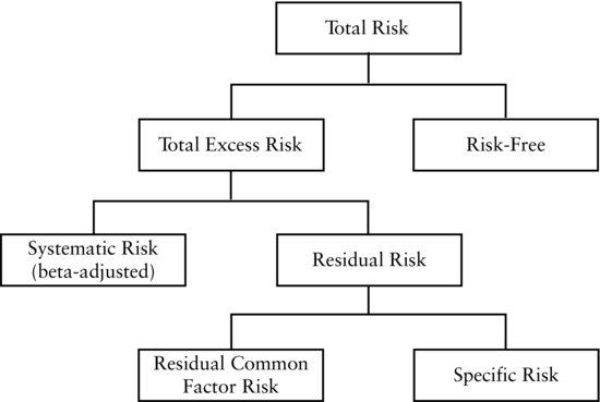
Figure 3 Active Risk Decomposition
Source: Figure 4.4 in Barra (1998, p. 34). Reprinted with permission.
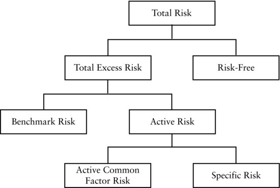
Residual risk in the systematic-residual risk decomposition is defined in a different way from residual risk in the total risk decomposition. In the systematic-residual risk decomposition, residual risk is risk that is uncorrelated with the market portfolio. In turn, residual risk is partitioned into specific risk and common factor risk. Notice that the partitioning of risk described here is different from that in the arbitrage pricing theory model where all risk factors that could not be diversified away were referred to as “systematic risks.” In the discussion here, risk factors that cannot be diversified away are classified as market risk and common factor risk. Systematic risk can be diversified to a negligible level.
Active Risk Decomposition
The active risk decomposition approach is useful for assessing a portfolio’s risk exposure and actual performance relative to a benchmark index. In this type of decomposition, shown in Figure 3, the total excess return is divided into benchmark risk and active risk. Benchmark risk is defined as the risk associated with the benchmark portfolio.
Figure 4 Active Systematic-Active Residual Risk Decomposition
Source: Figure 4.5 in Barra (1998, p. 37). Reprinted with permission.
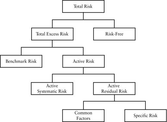
Active risk is the risk that results from the manager’s attempt to generate a return that will outperform the benchmark. Another name for active risk is tracking error. The active risk is further partitioned into common factor risk and specific risk. This decomposition is useful for managers of index funds and traditionally managed active funds.
Active Systematic-Active Residual Risk Decomposition
There are managers who overlay a market-timing strategy on their stock selection. That is, they not only try to select stocks they believe will outperform but also try to time the purchase of the acquisition. For a manager who pursues such a strategy, it will be important in evaluating performance to separate market risk from common factor risks. In the active risk decomposition approach just discussed, there is no market risk identified as one of the risk factors.
Since market risk (i.e., systematic risk) is an element of active risk, its inclusion as a source of risk is preferred by managers. When market risk is included, we have the active systematic-active residual risk decomposition approach shown in Figure 4. Total excess risk is again divided into benchmark risk and active risk. However, active risk is further divided into active systematic risk (i.e., active market risk) and active residual risk. Then active residual risk is divided into common factor risks and specific risk.
Summary of Risk Decomposition
The four approaches to risk decomposition are just different ways of slicing up risk to help a manager in constructing and controlling the risk of a portfolio and for a client to understand how the manager performed. Figure 5 provides an overview of the four approaches to carving up risk into specific/common factor, systematic/residual, and benchmark/active risks.
Figure 5 Risk Decomposition Overview
Source: Figure 4.6 in Barra (1998, p. 38). Reprinted with permission.
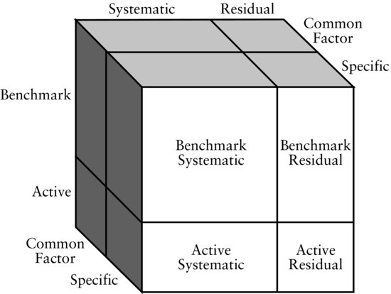
Table 2 Portfolio ABC’s Holdings (only the top 15 holdings shown)

APPLICATIONS IN PORTFOLIO CONSTRUCTION AND RISK CONTROL
The power of a multifactor risk model is that given the risk factors and the risk factor sensitivities, a portfolio’s risk exposure profile can be quantified and controlled. The three examples below show how this can be done so that a manager can avoid making unintended bets. In the examples, we use the Barra E3 factor model.4
A fundamental multifactor risk model can be used to assess whether the current portfolio is consistent with a manager’s strengths. Table 2 is a list of the top 15 holdings of Portfolio ABC as of December 31, 2008. Table 3 is a summary risk decomposition report for the same portfolio. The portfolio had a total market value of $5.4 billion, 868 holdings, and a predicted beta of 1.15. The risk report also shows that the portfolio had an active risk of 6.7%. This is its tracking error with respect to the benchmark, the S&P 500 index. Notice that nearly 93% of the active risk variance (which is 44.8) came from common factor variance (which is 41.6), and only a small proportion came from stock-specific risk variance (also known as asset selection variance, which is 3.2). Clearly, the manager of this portfolio had placed fairly large factor bets.
Table 3 Portfolio ABC’s Summary Risk Decomposition Report
| Number of Securities | 868 |
| Number of Shares | 298,371,041 |
| Average Share Price | $24.91 |
| Weighted Average Share Price | $35.30 |
| Portfolio Ending Market Value | $5,396,530,668 |
| Predicted Beta (vs. Benchmark, S&P 500) | 1.15 |
| Barra Risk Decomposition (Variance) | |
| Asset Selection Variance | 3.2 |
| Common Factor Variance: | |
| Risk Indexes | 22.5 |
| Industries | 11.7 |
| Covariance × 2 | 7.5 |
| Common Factor Variance | 41.6 |
| Active Variance | 44.8 |
| Benchmark Variance | 749.4 |
| Total Variance | 1,016.6 |
| Barra Risk Decomposition (Std. Dev.) | |
| Asset Selection Risk | 1.8 |
| Common Factor Risk: | |
| Risk Indexes | 4.7 |
| Industries | 3.4 |
| Covariance × 2 | |
| Common Factor Risk | 6.5 |
| Active Risk | 6.7 |
| Benchmark Risk | 27.4 |
| Total Risk | 31.9 |
Table 4 Analysis of Portfolio ABC’s Factor Exposures
The top portion of Table 4 lists the factor risk exposures of Portfolio ABC relative to those of the S&P 500 index, its benchmark. The first column shows the exposures of the portfolio, and the second column shows the exposures of the benchmark. The last column shows the active exposure, which is the difference between the portfolio exposure and the benchmark exposure. The exposures to the risk index factors are measured in units of standard deviation, while the exposures to the industry factors are measured in percentages. The portfolio had a high active exposure to the Volatility risk index factor. That is, the stocks in the portfolio were far more volatile than the stocks in the benchmark. On the other side, the portfolio had a low active exposure to the Size risk index. That is, the stocks in the portfolio were smaller than the benchmark average in terms of market capitalization. The lower portion of Table 4 is an abbreviated list of the industry factor exposures.
An important use of such risk reports is the identification of portfolio bets, both explicit and implicit. If, for example, the manager of Portfolio ABC did not intend to place the large bet on the Volatility risk index, then he has to make appropriate changes in the portfolio holdings until the active exposure to this factor is closer to zero.
Table 5 Factor Exposures of a 50-Stock Portfolio that Optimally Matches the S&P 500 Index
Risk Control against a Stock Market Index
The objective of equity indexing is to match the performance of some specified stock market index with little tracking error. To do this, the risk profile of the indexed portfolio must match the risk profile of the designated stock market index. Put in other terms, the factor risk exposure of the indexed portfolio must match as closely as possible the exposure of the designated stock market index to the same factors. Any differences in the factor risk exposures result in tracking error. Identification of any differences allows the indexer to rebalance the portfolio to reduce tracking error.
To illustrate this, suppose that an index manager has constructed a portfolio of 50 stocks to match the S&P 500 index. Table 5 lists the exposures to the Barra risk indexes of the 50-stock portfolio and the S&P 500 index. The last column in the exhibit shows the difference in exposures. The differences are very small except for the exposures to the Size risk index factor. Though not shown in this exhibit, there is a similar list of exposures to the 55 industry factors.
The illustration in Table 5 uses price data as of December 31, 2008. It demonstrates how a multifactor risk model can be combined with an optimization model to construct an indexed portfolio when a given number of holdings are sought. Specifically, the portfolio analyzed in the exhibit is the result of an application in which the manager wants a portfolio constructed that matches the S&P 500 index with only 50 stocks and that minimizes tracking error. The optimization model uses the multifactor risk model to construct a 50-stock portfolio with a tracking error versus S&P 500 index of just 2.75%. Since this is the optimal 50-stock portfolio to replicate the S&P 500 index with a minimum tracking error risk, this tells the index manager that if he seeks a lower tracking error, then more stocks must be held. Note, however, that the optimal portfolio changes as time passes and prices move.
Tilting a Portfolio
Now let’s look at how an active manager can construct a portfolio to make intentional bets. Suppose that a portfolio manager seeks to construct a portfolio that generates superior returns relative to the S&P 500 by tilting it toward low P/E stocks. At the same time, the manager does not want to increase tracking error significantly. An obvious approach may seem to be to identify all the stocks in the universe that have a lower than average P/E. The problem with this approach is that it introduces unintentional bets with respect to the other risk indexes.
Table 6 Factor Exposures of a Portfolio Tilted Toward Earnings Yield
Instead, an optimization method combined with a multifactor risk model can be used to construct the desired portfolio. The necessary inputs to this process are the tilt exposure sought and the benchmark stock market index. Additional constraints can be placed, for example, on the number of stocks to be included in the portfolio. The Barra optimization model can also handle additional specifications such as forecasts of expected returns or alphas on the individual stocks.
In our illustration, the tilt exposure sought is toward low P/E stocks, that is, toward high earnings yield stocks (since earnings yield is the inverse of P/E). The benchmark is the S&P 500. We seek a portfolio that has an average earnings yield that is at least 0.5 standard deviations more than that of the earnings yield of the benchmark. We do not place any limit on the number of stocks to be included in the portfolio. We also do not want the active exposure to any other risk index factor (other than earnings yield) to be more than 0.1 standard deviations in magnitude. This way we avoid placing unintended bets. While we do not report the holdings of the optimal portfolio here, Table 6 provides an analysis of that portfolio by comparing the risk exposure of the 50-stock optimal portfolio to that of the S&P 500. Though not shown in Table 6, there is a similar list of exposures to the 55 industry factors.
KEY POINTS
- There are three types of multifactor equity risk models that are used in practice: statistical, macroeconomic, and fundamental. The most popular is the fundamental model.
- A multifactor equity risk model assumes that stock returns (and hence portfolio returns) can be explained by a linear model with multiple factors, consisting of “risk index” factors such as company size, volatility, momentum, and so on, and “industry” factors. The portion of the stock return that is not explained by this model is the stock-specific return.
- The risk index factors are measured in standard deviation units, while the industry factors are measured in percentages.
- The real usefulness of a linear multifactor model lies in the ease with which the risk (i.e., the volatility) of a portfolio with several assets can be estimated. Instead of estimating the variance-covariance matrix of its assets, it is only necessary to estimate the portfolio’s factor exposures and the variance-covariance matrix of the factors, a computationally much easier task.
- The variance-covariance matrix of the factors and the factor exposures of stocks are calculated based on a mix of historical and current data and are updated periodically.
- Total risk of a portfolio can be decomposed in several ways. The partitioning method chosen is based on what is useful given the manager’s strategy. The active risk decomposition method is useful for managers of index funds and traditionally managed active funds.
- The level of active risk of a portfolio and the split of the tracking error variance between the common factor portion and the stock-specific portion are useful in assessing if the portfolio is constructed in a way that is consistent with the manager’s strengths.
- The list of active factor exposures of a portfolio helps the manager identify its bets, both explicit and implicit. If a manager discovers some unintended bets, then the portfolio can be rebalanced so as to minimize such bets.
- Using a multifactor risk model and an optimization model, a portfolio that has the minimum active risk relative to its benchmark for a given number of assets held can be constructed. This application is useful for passive managers.
- Similarly, a manager can construct a portfolio that tilts toward a specified factor and has no material active exposure to any other factor. This application is useful for active managers.
NOTES
1. For a discussion of the different types of factor models, see Connor (1995).
2. For a more detailed description of each descriptor, see Appendix A in Barra (1998). A listing of the 55 industry groups is provided in Table 4 in this entry.
3. See Chapter 4 in Barra (1998). The discussion to follow in this section follows that in the Barra publication.
4. The illustrations were created by the authors based on applications suggested in Chap-ter 6 of Barra (1996).
REFERENCES
Barra (1996). United States Equity Model Handbook. Berkeley, CA: Barra.
Barra (1998). Risk Model Handbook, United States Equity: Version 3. Berkeley, CA: Barra.
Connor, G. (1995). The three types of factor models. Financial Analysts Journal 15: 42–57.