
Introduction
This book deals with the concepts, methods, and algorithms of digital geometry. This introductory chapter provides a few basic definitions and a brief introduction to the subject; it discusses how digital geometry relates to other mathematic disciplines and indicates which related topics will and will not be covered in the book.
1.1 Pictures
Scientists often deal with functions defined in a space (e.g., in three-dimensional [3D] Euclidean space or in a lower-dimensional space such as a plane or a surface). Such functions are often obtained by collecting sensory data; for example, two-dimensional (2D) scanners collect data from a 2D surface; 3D sensors collect data from a volume of 3D space; and optical sensors collect 2D images by projecting a 3D scene onto a plane or surface. Because the functions are not always obtained using imaging processes, we will call them pictures rather than images.
When computers are used to process or analyze a 2D or 3D picture, they deal with a discrete form of the picture, obtained by a process of digitization, which involves sampling the picture and quantizing the sampled values. The resulting set of 2D or 3D digital data is called a digital picture. Picture analysis (more commonly called image analysis) derives multidimensional information about objects or scenes from sensory data. Conversely, computer graphics synthesizes and generates digital pictures from models for objects or scenes.
A 2D digital picture consists of a finite number of pixels, each of which is defined by a location and a value at that location. The term pixel is short for “picture element”; this acronym was introduced in the late 1960s by a group at Jet Propulsion Laboratory in Pasadena, California, that was processing pictures taken by space vehicles [640]. The analogous 3D term is “voxel,” which is short for “volume element.” In this book, we will use the terms pixel and voxel in a different sense; they will refer to the elements of the medium on which pictures reside, which is defined by a regular orthogonal grid. A picture is then a function defined on the grid that assigns values to the pixels or voxels. Thus, pixels and voxels are locations defined by grid coordinates, and they have values defined by a picture.
In this section, we introduce the standard methods of representing 2D digital pictures, in which a pixel is a grid point or a grid square. These representations, in both 2D and 3D, will be discussed in greater detail in Section 2.1.
1.1.1 Pixels, voxels, and their values
A 2D digital picture captured or constructed on a surface (usually planar) is typically defined using a finite data structure that models a regularly spaced planar orthogonal grid.
The values of pixels can be integers, floating point numbers, vectors, or even (finite) sets. For example, the values of pixels in color pictures are usually represented by triples of scalar values, such as red, green, and blue or hue, saturation, and intensity. For the purpose of this book, it will usually be sufficient to restrict pixel values to nonnegative integers.
A 3D picture is defined on a finite data structure that models a regular orthogonal grid in 3D space. We will sometimes also use one-dimensional (1D) pictures as simple examples. A 1D picture is defined on a (finite) set of regularly spaced points of a line. 2D or 3D pictures can also be defined on other grids; see Exercise 1 in Section 1.3 for the 2D case.
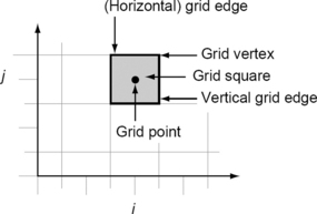
Pixels have grid-based coordinates; we assume integer coordinates as a default so that the regular planar orthogonal array can be identified with Z2= Z × Z = {(i,j)): i,j ∈ Z}, where Z is the set of all integers. Every grid point in Z2is the center point of a grid square with sides (grid edges) of length 1, oriented parallel to the Cartesian coordinate axes (see Figure 1.1). The corners of grid squares are called grid vertices. The corresponding terminology in 3D will be introduced in Section 2.1. Note that the assumption of a uniform orthogonal grid is a simplification. In practical applications (e.g., medical imaging), the spacing between pixels or voxels may vary. For example, a 3D magnetic resonance picture usually has larger spacing between slices (cross-sections) than within a slice; the units of measurement cannot be ignored in such situations. However, in digital geometry, the spacing between pixels is often not relevant.
A 2D grid of size m × n is a rectangular array of grid points
or a rectangular set of grid squares
where m,n > > 1 (read: “is much larger than 1”).
Figure 1.2 (left) shows a magnified small rectangular portion (sometimes called a “window”) of a picture. This illustrates the normal way pixels appear on a screen; after zooming in on a picture, the pixels are visible as colored squares, where the colors (or gray levels) represent the values of the pixels. In the common array data structure used to represent a picture, each pixel is represented by a pair of integers (i.e., by a grid point). Thus picture displays correspond to a grid composed of squares and array data structures to a grid composed of points (both types of grids coexist in picture analysis and computer graphics). We use both representations in this book as alternative ways of representing pictures.

Pictures are quantized as well as sampled; a pixel or voxel can have only a finite number of possible values. The range of values in a (scalar) picture P will usually be of the form {0,…, Gmax}, when 0 ≤ P (p) ≤ Gmax where Gmax ≥ 0. Gmax = 0 is the trivial case of a constant (“blank”) picture. (As mentioned earlier, the values in a color picture are triples [u1, u2, u3], such as red, green, and blue color components. These triples could also be mapped onto {0,…, Gmax}, but color is of no relevance in this book, so we can think of G as short for “gray level.” Color is becoming increasingly important in modern treatments of picture analysis and computer graphics, and it may also become more important in digital geometry. However, for the present, this book deals only with scalar (integer valued) pictures.
The range of values of the pixels or voxels in a binary picture1. is {0, 1} (i.e., Gmax = 1). The pixels whose values are 1 (called 1s for short) define a subset ![]() of the grid. These pixels are often referred to as “object” or “black” pixels. (In multivalued pictures, higher pixel values usually correspond to lighter gray levels, with gray level 0 being black; the opposite convention is often used for binary pictures: black = 1, white = 0.) Nonobject pixels in
of the grid. These pixels are often referred to as “object” or “black” pixels. (In multivalued pictures, higher pixel values usually correspond to lighter gray levels, with gray level 0 being black; the opposite convention is often used for binary pictures: black = 1, white = 0.) Nonobject pixels in ![]() are called 0s for short.
are called 0s for short.
1.1.2 Picture resolution and picture size
Picture resolution is a display parameter. It is defined in dots per inch (dpi) or equivalent measures of spatial pixel density, and its standard value for recent screen technologies is 72 dpi. Recent printers use resolutions such as 300 dpi or 600 dpi, and such values can also be used for picture presentation on a screen.
Picture resolution is also a digitization parameter that is measured in samples per inch or equivalent measures of spatial sampling density. The human eye itself makes use of sampled pictures. The retina of the eye is an array of about 125 million photoreceptor cells called rods and cones. A rod is about 0.002 mm in diameter, and a cone is about 0.006 mm in diameter.
Pictures whose acquisition satisfies the traditional pinhole camera model are captured on planar surfaces. The light-sensitive array of a typical digital camera, which is a charge-coupled device (CCD) matrix, can be regarded as a rectangular set of square cells in a plane. The elements of the matrix capture a discrete set of pixel values. Other types of cameras may capture pictures on nonplanar surfaces. For example, Figure 1.3 shows a super–high-resolution panoramic picture captured with a rotating line camera. A geometric model of the panoramic picture acquisition process assumes that the picture is captured on a cylindric surface.

FIGURE 1.3 A 380° panoramic picture of Auckland, New Zealand, captured from the top of the harbor bridge. The full-resolution picture consists of about 104 × 5 · 104 pixels captured on a cylindric surface with a rotating line camera.
Discrete methods of picture generation are frequently used in both art and technology. The dots in a pointillistic painting can be as small as 1/16 of an inch in diameter. Figure 1.4 illustrates two other technologies for discrete picture generation: pebble mosaics or tiled floors are composed of pixels, and patterns on fabrics or rugs can also be regarded as digital pictures. In 1725, B. Bouchon invented the idea of controlling a loom by perforated tape. The pattern generated by the loom was broken up into discrete areas with discrete color values. This idea was further developed by Falcon, a master silk weaver in Lyons, France. In 1738, Falcon applied for an English patent on his automatic card-controlled loom and provided a small working model as was required by English patent law. That working model continues to operate in the Science Museum in London, driven by an electric motor and weaving threads of several colors into patterned ribbon with the pattern controlled by punched cards laced together in a loop. When Falcon died in 1765, about 40 of his looms were operating. J.-M. Jacquard greatly improved the design of card-controlled looms in the early 19th century; thousands of Jacquard looms were soon in operation [835]. Thus pictures were generated by a programmed machine even before the first programmed machine (invented by C. Babbage) performed calculations on numbers! A surviving example of a pattern woven by a Jacquard loom is a black-and-white silk portrait of Jacquard himself, woven under the control of a “program” consisting of about 24,000 cards.

FIGURE 1.4 Lower left: a Greek pebble mosaic, detail from “The Lion Hunt” in Pella, Macedonia, circa 300 BC. Right and top: a picture of J.-M. Jacquard woven on silk on one of his “programmable” looms by digitizing a portrait of him, and one of the 24,000 punched cards that controlled the loom [669].
Today we think of pixels as tiny cells on a screen or as atomic units of a digital picture stored on a CD or DVD or in a computer. New media for representing large quantities of pictorial information will become available in the future, and contemporary screen technology may seem like pebbles only a few years from now.
Picture size is another important picture property. Pictures cannot be arbitrarily large; picture capturing, display, and printing technologies will always impose finite limits. The number of pixels in a typical picture has increased greatly since the early days of picture analysis and computer graphics (the 1950s and 1960s). In those days, a picture might contain only a few thousand pixels; today, a color picture may require gigabytes of memory, as we saw in Figure 1.3.
1.1.3 Scan orders
Algorithms in picture analysis are often applied to the pixels of a picture in sequence, where the sequence is obtained by scanning the grid. A scan of a grid Gm,n is a one-to-one mapping φ of the m × n pixels of the grid into a linear sequence φ(1), …φ (mn). Scans are used in picture processing programs to control the order of pixel accesses. A scan can also be viewed as an enumeration of the pixels; φ(k) is the k-th pixel (1 ≤ k ≤ mn).
G. Cantor (1845–1918) showed, using his famous enumeration principle, that the set of all rational numbers has the same cardinality ![]() as the set of all natural numbers (i.e., this set is infinite but still enumerable). The enumeration scheme shown in Figure 1.5 defines a scan of the infinite set Z2 of grid points.
as the set of all natural numbers (i.e., this set is infinite but still enumerable). The enumeration scheme shown in Figure 1.5 defines a scan of the infinite set Z2 of grid points.
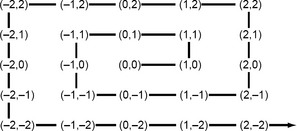
FIGURE 1.5 Enumeration principle defining a scan of the infinite grid, starting at (0,0) and proceeding in outward spiral order.
The standard method of scanning a grid Gm,n is row by row, with the pixels in each row accessed from left to right and the rows accessed from top to bottom; this scan order is often called row-major order. It is a lexicographic order derived from the grid coordinates: (1, 1), (1, 2),…, (1,n), (2, 1), (2, 2),… in the 2D case, where (1, 1) is in the upper left-hand corner; (i1, j2) < (i1, j2) iff2 i1 < i2, or i1 = i2 and j1 < j2. 3D scan order is defined analogously. This and five other common scan orders are illustrated in Figure 1.6. Standard and reverse standard scans are used, for example, for defining distance transforms in Section 3.4. Selective scans can be applied, for example, to speed up the search for picture objects when an estimate of the minimum size of the objects is available. In general, a scan can be split into scans of even rows followed by scans of odd rows, and this splitting process can be repeated recursively.
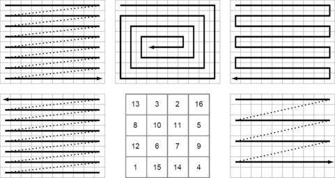
FIGURE 1.6 Scan orders: standard (upper left), inward spiral (upper middle), meander (upper right), reverse standard (lower left), magic square (lower middle), and selective, as used in interlaced scanning: standard, every second row (lower right).
Scan orders play only minor roles in digital geometry, but they can be of interest in discrete mathematics. For example, the magic-square scan is an enumeration of pixels such that the sums of the pixel numbers in each row and column are equal. This scan is easily constructible for small pictures, and its scan order may appear to be “pseudorandom.” Random scans can be defined using a random number generator to address one pixel at a time. (Efficiently keeping track of the set of remaining pixels is an interesting algorithmic problem.)
Scans related to the mathematic history of defining curves have also found their way into the picture-processing literature. This historic context may justify our briefly discussing two examples of “space-filling” curves: the Peano curve and the Hilbert curve.
The Peano curve was originally defined by G. Peano (1858–1932) in 1890, following a proposal by C. Jordan about a method of defining curves in parametric form. Peano showed that a curve defined in that form can completely fill a square, and Jordan therefore revised his original definition. Figure 1.7 illustrates a recursive (nonparametric) way of constructing the Peano curve by infinite repetition of the construction. Of course, in practice, we use only finitely many repetitions of the construction, in a grid of size 3n × 3n; the resulting curves are called Peano scans.
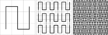
FIGURE 1.7 Peano scan: The scan pattern on the left is repeatedly used (nine times) to obtain the refined scan in the middle (with rotations at some places), and the same pattern of repetition of the scan in the middle is used to obtain the scan on the right.
In 1891, D. Hilbert defined a similar curve. A finite number of repetitions of this construction, as illustrated in Figure 1.8, leads to a Hilbert scan in a grid of size 2n × 2n.

FIGURE 1.8 Hilbert scan: The scan pattern on the left is repeated only four times (with rotations) to obtain the refined scan.
Any scan of a binary picture defines runs of 0s and 1s: maximum-length sequences of 0s or 1s that are visited by the scan. Evidently, runs of 0s must alternate with runs of 1s, and each run has a length of at least 1.
1.1.4 Adjacency and connectedness
Grid points are isolated points in the (real) plane, but, in the grid, adjacency relations between grid points can be defined. For p = (x,y)∈ Z2, we define the neighborhoods
and
Two grid points p,q ∈ Z2are called 4-adjacent or proper 4-neighbors (8-adjacent or proper 8-neighbors) iff p ≠ q and p ∈ N4(q) (p ∈ N8(q)). We often use geographic language to identify the proper neighbors of a pixel: (x,y + 1) is called the north neighbor, (x + 1, y + 1) is called the northeast neighbor, and so on.
Neighborhoods can also be defined for grid squares by applying 4- or 8-adjacency to the center points (grid points) of the grid squares, and they can also be defined for grids in 3D space. Adjacency relations in 2D and 3D grids will be discussed in greater detail in Chapter 2.
The reflexive, transitive closure of an adjacency relation on a set M (e.g., of grid points), which is the smallest reflexive, transitive relation on M that contains the given adjacency relation, defines a connectedness relation. M is called connected if for all p,q ∈ M there exists a sequence p0,…, pn of elements of M such that p0 = p, pn = q, and pi is adjacent to pi−1(1 ≤ i ≤ n); such a sequence is called a path and is said to join p and q in M. Maximal connected subsets of M are called (connected) components of M. Evidently, components are nonempty and distinct components are disjoint. The concepts of 4- and 8-adjacency, connectedness, and components were introduced into picture analysis in 1966 [921], although the prefixes “4-” and “8-” were not used until a few years later.
It was observed in [921] that difficulties arise when 4-adjacency or 8-adjacency (and the corresponding type of connectedness) is used for both the 1s and 0s in a binary picture. Figure 1.9.a (an object containing two pixels) is 8-connected, as is its complementary set. Figure 1.9.b is both 4- and 8-connected, and its complement is neither 4- nor 8-connected. Figure 1.9.c is neither 4- nor 8-connected, but its complement is both 4- and 8-connected.
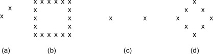
FIGURE 1.9 Examples of connected and nonconnected sets [921]. The xs stand for 1s; the 0s are not shown.
“The ‘paradox’ of Figure 1.9.d can be (expressed) as follows: If the ‘curve’ is connected (‘gapless’) it does not disconnect its interior from its exterior; if it is totally disconnected it does disconnect them. This is of course not a mathematical paradox,3 but it is unsatisfying intuitively; nevertheless, connectivity is still a useful concept. It should be noted that if a digitized picture is defined as an array of hexagonal, rather than square, elements, the paradox disappears.” [921]
The first case assumes 8-connectedness for both “curve points” and “background points,” and the second case assumes 4-connectedness for both.
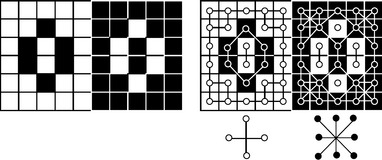
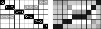
Commenting on [921] (in an unpublished technical report in 1967), R.O. Duda, P.E. Hart, and J.H. Munson proposed the dual use of 4- and 8-connectedness for 0s and 1s in a binary picture [286]. Figure 1.10 illustrates the use of 4-adjacency for white pixels and 8-adjacency for black pixels in a binary picture. The advantages of using opposite types of adjacency for the 0s and the 1s in binary pictures will be discussed in later chapters.
1.2 Digital Geometry and Related Disciplines
We usually assume that objects are represented by connected sets of pixels or voxels and that the quantitative information involves quantities studied in Euclidean or similarity geometry (see Section 1.2.2); we can then attempt to ensure that the properties computed in digital geometry adequately approximate these quantities. In this sense, we can regard digital geometry as digitized similarity geometry. As we will see in Section 1.2.2, Euclidean geometry is a special case of similarity geometry.
Digital geometry also often attempts to obtain topologic characterizations of pictures or to transform pictures into “simpler” topologically equivalent pictures. Due to the discrete nature of digital geometry, these topologic problems belong to the field of combinatorial topology (the topology of cell complexes), which is discussed in Chapter 6.
The remainder of this section briefly discusses topics and disciplines related to digital geometry and indicates the extent to which these topics will be treated in this book.
1.2.1 Coordinates and metric spaces
The concept of defining the locations of points in a plane by their distances from two straight lines (“axes”) was used by Archimedes and Apollonius more than 2000 years ago. A Cartesian coordinate system makes use of a set of axes as introduced by R. Descartes (in Latin: Cartesius, 1596–1650) in [264] to define nonnegative coordinates in the plane. Descartes dealt with general oblique coordinates, addressing rectangular coordinates as an important special case.4 Negative coordinates were first proposed by I. Newton, and the first use of the term “coordinates” is ascribed to G. Leibniz. When we use rectangular Cartesian coordinates, we define the (real) plane as a “Cartesian product” of two (real) lines: R2 = R × R, where R is the set of reals. A Cartesian coordinate system in the plane, together with the Euclidean metric (see p. 12), defines the Euclidean plane E2. The n-dimensional real and Euclidean spaces are defined analogously using n-fold Cartesian products. The point o where the axes intersect is called the origin of the coordinate system; because o is at distance 0 from all the axes, its coordinates are all 0s.
A right-handed coordinate system is a rectangular Cartesian coordinate system in which the positive x-axis is identified with the thumb (pointing outward in the plane of the palm), the positive y-axis with the forefinger (pointing outward in the plane of the palm), and, in 3D, the positive z-axis with the middle finger of the right hand (pointing downward from the plane of the palm).
Coordinate systems can also be defined using distances to points. For example, barycentric coordinates (homogeneous or triangular coordinates) in the plane were introduced by Möbius in 1827 [807] as a way of representing points in the plane relative to a given triple of noncollinear points. The prefix bary- refers to weight or mass. For any point p inside the triangle, there exist masses a, b, and c such that, if they are placed on the vertices of the triangle, their center of gravity (balancing point) will be at p. The masses a, b, and c are uniquely determined if we require that a + b + c = 1. The triple (a, b, c) defines the barycentric coordinates of p in the given triangle.
The measurements studied in picture analysis are always related to a regular grid that defines the locations of pixels or voxels in a Cartesian coordinate system. If we fix all but one of the coordinates, the locations become regularly spaced points on a line. The distance between consecutive locations on such a line is called the grid constant; it is the unit or scale of measurement in the grid coordinate system.
Let S be an arbitrary nonempty set. A function d: S × S → R is a distance function or metric on S iff it has the following properties:
M1: For all p,q ∈ S, we have d(p, q) ≥ 0, and d(p, q) = 0 iff p = q (positive definiteness).
M2: For all p,q ∈ S, we have d(p, q) = d(q,p) (symmetry).
M3: For all p,q,r ∈ S, we have d(p,r) ≤ d(p,q) + d(q,r) (triangularity: the triangle inequality).
If d is a metric on S, the pair [S, d] defines a metric space. M. Fréchet (1878–1973) introduced the concept of a metric space; the elements of S can be any mathematic objects. The name “metric space” is due to F. Hausdorff (1868–1942). Quantitative geometric measurements are often based on metrics.
It should be pointed out that property M1 can be simplified to the following:
M1: For all p,q ∈ S, we have d(p, q)= 0 iff p = q.
Indeed, from the simplified M1 together with M2 and M3, we have as follows:
0 = d(p,p) ≤ d(p, q) + d(q, p) = 2d(p, q) for all p, q ∈ S
Let [S, d] be a metric space, p ∈ S, and ∈ > 0. The set of points q ∈ S such that d(p, q) ≤∈ is called a ball of radius∈ with center p. A subset M of S is called bounded iff it is contained in a ball of some finite radius.
Euclidean space En is defined with an orthogonal coordinate system; it is used to define a metric de called the Euclidean metric. If two points p, q have coordinates (xl,…, xn) and (y1,…, yn), we define the following:
It will be proved in Chapter 3 that de is a metric. Two-dimensional Euclidean space is called the Euclidean plane E2is a subspace of E2, which is defined by the subset of all points with integer coordinates and the Euclidean metric; Z2is the digital plane.
Metrics defined on grids or on Euclidean spaces play central roles in digital geometry. They will be frequently used in this book and will be discussed in detail in Chapter 3.
1.2.2 Euclidean, similarity, and affine geometry
The history of geometry dates back about 4000 years to societies in Egypt, Mesopotamia, and China. The word geometry, which means earth measurement, has been in use for more than 2500 years. The measurement of distances and the calculation of areas and volumes are among the earliest developments in mathematics. Of course, only simple 2D or 3D objects such as polygons, prisms, cuboids, and cylinders were studied in those days.
A (finite, connected) polygonal arc in Euclidean space En is a finite sequence of points (p1, p2,…, pn) where n ≥ 3, which defines n−1 straight line segments pipi+1. (i = 1,2,…, n−1). The pis are called the vertices of the arc, and the line segments are called its edges. The polygonal arc forms a circuit ![]() if we add the nth edge pnp1.
if we add the nth edge pnp1.
A simple polygon Π= ![]() (an “n-gon”) is a polygonal circuit such that no point belongs to more than two edges and the only points that belong to two edges are the vertices; see Figure 1.11. If n = 3, the polygon is called a triangle.
(an “n-gon”) is a polygonal circuit such that no point belongs to more than two edges and the only points that belong to two edges are the vertices; see Figure 1.11. If n = 3, the polygon is called a triangle.
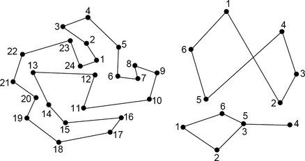
FIGURE 1.11 A simple planar polygon (left) and two nonsimple planar polygons (right). The numbers specify a cyclic order of the vertices.
The concept of an angle, the decomposition of a simple planar polygon into triangles, and the calculation of simple areas and volumes (such as the volume of a frustum of a pyramid) were known in ancient Egypt. The law of Pythagoras (about right triangles) was known in ancient Mesopotamia, and the laws of similar triangles were also widely used.
It is not certain whether Euclid of Alexandria (about 325–265 BC) was an individual, the leader of a team of mathematicians, or the pseudonym of a group of mathematicians. It is certain, however, that the book The Elements established Euclidean geometry on the basis of just a few postulates (or “axioms”) about straight lines, straight line segments, circles, and angles.
Similarity and affine geometry are “intermediate” between Euclidean and projective geometry (see Section 1.2.3) with respect to the transformations that are allowed (see Table 1.1) and the quantities or relations that remain invariant under these transformations (see Table 1.2).5 The use of invariants under groups of transformations to characterize geometries will be discussed in Chapter 14.


In general, the transformations listed in Table 1.1 do not take grids into themselves. For example, a rotation takes an orthogonal grid into itself only if it is a rotation by a multiple of 90°. The application of general transformations to a grid requires approximation or interpolation, as discussed in Chapter 14. As a result, the “invariants” listed in Table 1.2 are only approximately invariant when the transformations are applied to digital pictures.
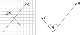
Objects in digital geometry often do not behave like Euclidean objects. For example, we can define adjacency relations between pixels (see Section 1.1.4), whereas distinct points cannot be “adjacent” in Euclidean geometry. Digital lines are sequences of pixels and can intersect in segments (see Figure 1.12, left). Nonparallel lines may have no pixel in common; if two lines are defined by sequences of 8-adjacent pixels, they can cross without intersecting. The two digital “arcs” and the digital “ellipse” on the right in Figure 1.12 have no pixel in common!
1.2.3 Projective geometry
In the fifteenth century, some Italian painters developed a system of perspective that allowed them to paint the world as it is seen. This inspired new geometric ideas and led G. Desargues (1596–1662) to invent projective geometry.
A picture acquisition process that maps (the visible portion of) a scene onto a surface has an ideal description in terms of projective geometry (see Figure 1.13). In actual digital pictures, the pixels vary from this ideal (e.g., in the case of a planar picture because of the finite physical dimensions and small irregularities of the cells of the CCD array; in the case of a cylindric picture [see Figure 1.3] because of rotation errors of the line camera; and in both cases because of optical aberrations).
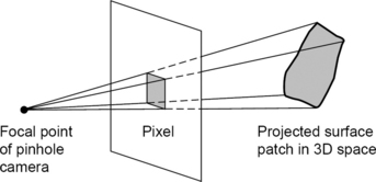
If we use the ideal description, the geometric resolution of a picture is specified by the geometric laws of projection that model the picture acquisition process. Geometric resolution allows us to relate measurements in pictures (in terms of pixel coordinates) to measurements in the real world. Picture resolution, which was discussed in Section 1.1.2, is a display parameter that need not correspond to geometric resolution.
A CCD cell in a camera collects light from a scene or object surface patch (see Figure 1.13). The size of this patch depends on the size of the cell, the camera optics (e.g., focal length, aberrations), the distance and direction between the camera and the surface of the object, and the 3D shape of the object. Thus geometric resolution depends on many picture acquisition parameters. Camera calibration, which is a subject in the computer vision literature, deals with the calculation of these parameters.
If a picture shows only a flat surface (e.g., a document, a microscope slide), specification of the picture size and the pixel size or spacing in terms of coordinates on the surface is relatively simple. Similar remarks apply to aerial pictures obtained by a camera flying at constant altitude over flat terrain. In such situations, picture resolution has a simple relationship to geometric resolution, so measurements made on the picture can be easily related to geometric measurements made on the surface.
In a 3D scene such as the head of the Gauss statue in Figure 1.14, the problem of calculating geometric resolution is much more complicated. Different pixels in the picture may correspond to surface patches of different sizes in the scene. Determining these sizes may require 3D shape recovery and the application of projective geometry to map the pixels onto the recovered surface. This book will not discuss camera calibration, 3D shape recovery, or projective geometry, and it will not deal with modeling picture acquisition processes in a 3D environment. The reader is referred to books about computer vision that deal with these subjects.
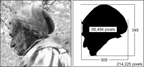
FIGURE 1.14 Left: detail of the Gauss statue in Göttingen, Germany. Right: number of pixels in the area of the head and in the entire picture, and height and width measured in numbers of pixel units (grid edges).
Both geometric and picture resolution have increased over the years because of progress in picture acquisition and display technologies. In this book, we will normally not be concerned with geometric picture size or resolution but only with the sizes of pictures as measured in numbers m × n of pixels.
1.2.4 Vector and geometric algebra
A grid point p can be identified with a vector ![]() that starts at the origin o and ends at p; we can also consider vectors
that starts at the origin o and ends at p; we can also consider vectors ![]() from one grid point to another. In this book, we deal only with 2D and 3D pictures. (We do not consider time sequences of 2D or 3D pictures as being 3D or 4D pictures in which the last coordinate is time; the time coordinate is qualitatively different from the spatial coordinates.) However, we will sometimes use n-dimensional spaces in this book (e.g., as a generalization of 2D and 3D spaces or when we deal with n-tuples of property values).
from one grid point to another. In this book, we deal only with 2D and 3D pictures. (We do not consider time sequences of 2D or 3D pictures as being 3D or 4D pictures in which the last coordinate is time; the time coordinate is qualitatively different from the spatial coordinates.) However, we will sometimes use n-dimensional spaces in this book (e.g., as a generalization of 2D and 3D spaces or when we deal with n-tuples of property values).
The 2D vector space [R2, +, ·, R] over the real numbers is defined by an addition operation (x1, x2) + (y1, y2) = (x1 + y1, x2 + y2) for all (x1, y1), (x2, y2) in R2 and a scalar multiplication operation a · (x,y) = (ax, ay) for all a ∈ r and all (x,y)∈ R2. Higher-dimensional vector spaces are defined analogously using n-tuples rather than pairs.
A vector space [S, +, ·, R] over the real numbers R is defined by a nonempty set S and two operations, + and ·, that have the following properties for all p,q,r ∈ S and all a, b ∈ R:
V0: p + q ∈ S and a · p ∈ S (closure under vector addition and under scalar multiplication)
V1: p + q = q + p (commutativity of vector addition)
V2: (p + q) + r = p + (q + r) (associativity of vector addition)
V3: a · (b · p)=(ab) · p (associativity of scalar multiplication)
V4: (a + b) · p = a · p + b · p (distributivity of scalar multiplication over vector addition)
V5: a · (p + q) = a · p + a · q (distributivity of vector addition over scalar multiplication)
V6: There exists an o ∈ S such that o + p = p (identity for vector addition).
V7: 1 · p = p (identity for scalar multiplication)
V8: For any p ∈ S, there exists −p ∈ S such that p + (–p) = o (inverse for vector addition).
A vector space is called finite-dimensional if there exists a finite subset B of S such that every p ∈ S is a sum of scalar multiples of vectors in B. S is called n-dimensional if the smallest such B has cardinality n. The elements of S are called vectors, and the elements of R are called scalars.
The norm || p || of a vector p = (x1,…, xn)∈ Rn is as follows:
Note that ||p|| = 0 iff x1 = … = xn = 0; evidently this implies that p = o. If p ≠ o, the direction of p is defined by the unit vector p° = p/||p||.
The dot product of p = (x1,…, xn) and q = (y1,…, yn) is as follows:
It can be shown that
where η is the (smaller) angle between the unit vectors p° and q°, 0 ≤ η < π.
p and q are called orthogonal iff p·q = 0, and they are called orthonormal iff they are orthogonal and |p| = |q| = 1.
The cross product will be defined here only for n = 3:
It can be shown that if p and q are linearly independent (i.e., there do not exist a,b ∈ R, a ≠ 0, and b ≠ 0 such that ap + bq = 0); then p × q is orthogonal to the plane defined by p and q. We also have
Vector algebra can be generalized to multidimensional oriented geometric entities such as are studied in Clifford or geometric algebra; see [772] for a review of the work by W.K. Clifford (1845–1879). This theory is based on definitions of “inner” and “outer” products of “multivectors,” which are classified by their “grades.” (The inner product generalizes the dot product. Multivectors of grade 0 are scalars in R; of grade 1 are vectors in Rn [n ≥ 2]; of grade 2 are bivectors that are oriented trapezoids defined by the outer product of two vectors; of grade 3 are oriented volume elements; and so forth.) Geometric algebra allows compact descriptions of distances and “angles” between geometric entities, including “degrees of parallelism.” Related studies in digital geometry might be of future interest, but the subject is not forth discussed in the present edition. As a possible initial step, see Chapter 3 for digital versions of the definitions of angles and seminorms.
1.2.5 Graph theory
Euler’s analysis of the bridge situation in Königsberg, Germany (i.e., is it possible to cross all of the bridges just once during a walk through the city?) initiated graph theory. The Königsberg bridge situation is shown in Figure 1.15; for more about the solution to the problem (i.e., the nonexistence of such a walk), see Section 4.1.1.
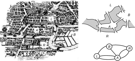
FIGURE 1.15 Three different representations of the Königsberg bridge situation. Left: The city at the time of Euler. Right, top: Simplified map (not to scale) of the islands, the left and right banks of the river, and the bridges. Right, bottom: Schematic representation; the labeled circles represent the islands and banks, and the arcs represent the bridges.
An adjacency relation, for example, on grid points (see Section 1.1.4), defines an undirected graph whose nodes are the grid points and where there is an edge between two nodes iff the corresponding grid points are adjacent. Graphs will be discussed in Chapter 4.
A path of length n in a graph is a finite sequence of nodes p0,….pn such that there is an edge betweenpi and pi−1 (1 ≤ i ≤ n). If such a path exists, we say that p0 and pn are connected. (Evidently connectedness is symmetric, because the reversal of a path from p to q is a path from q to p; it is also transitive, because, if there are paths from p to q and from q to r, we obtain a path from p to r by concatenating the two paths.) We also say that each node is connected to itself by a path of length zero; thus connectedness is reflexive as well as symmetric and transitive. A set of nodes of a graph is connected iff every pair of its nodes is connected. For example, the graph on the right in Figure 1.10 is not connected.
A maximal connected set of nodes of a graph is called a (connected) component. For example, the graph on the right in Figure 1.10 has eight components. A connected graph consists of a single component. Finite components (with respect to a given adjacency relation) of the pixels of voxels of a picture are called regions. Digital geometry is often concerned with geometric properties of regions.
Graph theory deals with many topics that are not directly relevant to digital geometry. However, many topics in digital geometry can be discussed on a graph-theoretic level, treating pixels or voxels as nodes of a graph rather than as elements of a grid. In Chapter 4 we will emphasize graph-theoretic concepts that are applicable to digital geometry.
1.2.6 Topology
The origin of topology is often identified with the Descartes-Euler Theorem α0 −α1 +α2 = 2, which was originally stated regarding the numbers α2,α1, and α0 of faces, edges, and vertices of a convex polyhedron. (A convex polyhedron is a nonempty bounded set that is an intersection of finitely many half-spaces.)
J.B. Listing (1802–1882) was the first to use the word “topology” in his correspondence, beginning in 1837.6 The term, which replaced Leibniz’s “geometria situs” or “analysis situs,” was introduced to distinguish “qualitative geometry” from geometric topics that emphasized quantitative measurements and relations. Topology can be informally viewed as “rubber-sheet geometry”: the study of properties of objects that remain the same when the objects are (continuously) deformed. For example, incidence relations between sets are topologically invariant.
As a more specialized example of a topologic property, the genus of a connected set is the minimum number of “cuts” needed to transform the set into a simply connected set.7 The 3D object shown in Figure 1.16 has genus 3 (the complexity of this example illustrates the advanced concepts that were being studied in topology even at its birth in the mid-19th century); the three 2D objects shown in Figure 1.17 have genus 0, 1, and 2, respectively. Genus is a qualitative property that characterizes the degree of connectedness of a set. Aspects of topology that are relevant to digital geometry will be reviewed in Chapters 6 and 7.
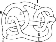
FIGURE 1.16 Positions of possible cuts in a 3D solid [660].

Digital topology (see Chapters 6 and 7.) provides topologic foundations for digital geometry. It extends the graph-theoretic concepts mentioned in Section 1.2.5 and develops a topologic theory of subsets of pictures that provides a basis for designing many algorithms for 2D and 3D picture analysis.
1.2.7 Approximation and estimation
The fundamental theorem of approximation theory is due to K.W.T. Weierstrass (1815–1897). It states that, for any function f that has continuous derivatives on a finite interval [a, b] and for any ε < 0, there exists a polynomial g such that | f (x) – g(x)| < ∈ for all x ∈ [a,b]. This illustrates the orientation of approximation theory toward continuous functions, polynomials, and arbitrarily small errors. Digital geometry differs from approximation theory in all of these respects: digital data need not be obtained from continuous functions; approximations usually involve linear functions such as straight line segments or planar surface patches; and the approximations may not be arbitrarily close.
Approximation is commonly used to estimate the values of geometric quantities. In ancient mathematics, Archimedes estimated π on the basis of inner and outer regular n-gon approximations of a circle with n = 3, 6, 12, 24, 48, 96; see the left side of Figure 1.18. (An n-gon is called regular if its edges all have the same length.) For n = 6, this approximation gives 3 < π < 3·46; for n = 96, it gives the following:

FIGURE 1.18 Inner and outer 6-gons approximating a circle, and percentage errors between the perimeters of the inner n-gons and the perimeter of the circle.
In this method of approximation, the perimeters p of the inner and outer regular n-gons converge toward the circle’s perimeter as n → ∞. For example, let the radius of the circle be r so that its perimeter is 2πr, and let the inner nm-gon Pnm have nm = 3 × 2m edges of length em so that P (Pnm) = nm · em. From elementary geometry
where e0 = ![]() for a triangle, e1 = r for a hexagon, and so on. It follows that the estimation error
for a triangle, e1 = r for a hexagon, and so on. It follows that the estimation error
converges to zero as nm → ∞ (see the right side of Figure 1.18; e.g., κ(3)/P(P3.) = 17·3028… andκ(24)/P(P24) = 0·2853…). The speed of convergence 1/κ(n) is thus (asymptotically) a linear function of n.
An improved method of calculating π was given by the Chinese mathematician Liu Hui in 263. He calculated the areas Sn of regular n-gons inscribed in a circle and proved that, for all n > 2, the area S of the circle is bounded by S2n < S < S2n + (S2n – Sn). Starting with n = 6, he doubled n five times to 192 and got close bounds for the area S. From that area, he computed the circumference of the circle and got an approximation to π of 3·1410 [1148].
These historic examples of length estimation by approximation do not fit into the methodologic framework of digital geometry. The inner regular nm-gons are defined by sample points on the circle, and the outer regular nm-gons are defined by tangent lines to the circle. In digital geometry, we cannot use such samples, which can be arbitrary points and lines in the Euclidean plane and have exact relationships with the circle; we have to deal with sets of grid points, which are not arbitrary points and need not exactly lie on the circle (“digitization error”).
A common task in 2D image analysis is to find a curve (e.g., an ellipse) that best fits (with respect to some error criterion) a given set of pixels. Figure 1.19 shows a best-fitting ellipse constructed using a numeric method described in [329]. Note that this ellipse does not necessarily circumscribe the set of pixels. Numeric methods are not discussed in this book, except for an iterative (3D) curve approximation algorithm in Chapter 10.

FIGURE 1.19 Left: a picture of a pupil. Middle: the set of pixels detected as the edge of the pupil. Right: the ellipse fitted to these pixels.
The estimates of geometric quantities studied in this book will be based only on digital approximations. A methodology for studying the convergence of digital approximations to geometric quantities as the grid constant goes to zero will be described in Section 2.4.
1.2.8 Combinatorial geometry
Generalizations of Archimedes’ and Liu Hui’s methods of estimating perimeter are studied in combinatorial geometry, which is more than 100 years old; it started with the geometry of numbers established by H. Minkowski (1864–1909). The geometry of numbers does not have close links with digital geometry in spite of the use of grid points in both fields. However, some results in combinatorial geometry are potentially applicable to digital geometry, especially if they deal with sets of grid points. Examples that we will discuss in this book are corner counts for isothetic polygons or polyhedra8 and asymptotic bounds on the number of convex grid polygons in an m × n grid. We also apply (in Chapter 9) the Transversal Theorem [957], which is a direct consequence of Helly’s First Theorem [422]:
Let F be a finite family of parallel straight line segments in R2. If every three segments in F have a common transversal, then there is a transversal common to all of the segments in F.
A transversal of a straight line segment σ in R2 is a straight line that intersects σ but does not contain it.
We give two recent examples [789] of results in combinatorial geometry. Let A(S) denote the area of a bounded subset S of the plane. Let S be convex and have nonzero area. (A set S is called convex if for any two points p, q of S the straight line segment pq is contained in S.) Let ∏n (πn), where n ≥ 3, be an n-gon of minimum area circumscribed around S (of maximum area inscribed in S). The sequence of positive reals A(∏n) (A(πn)) decreases (increases) as n → ∞. Furthermore, we have
for all n ≥ 4; hence, if A(∏m) = A(∏m+1) (A(πm) = A(πm+1)), then A(∏n) = A(∏m) (A(πn)= A(πm)) for all n ≥ m.
Similarly, let P(S) denote the perimeter of a bounded subset S of the plane. (We assume that the frontier of S is rectifiable so that its perimeter is well defined. Measurability and rectifiability will not be defined in this book; the frontier of a set will be defined in later chapters.) Let S be convex and have nonzero area. Let ∧n (λn), where n ≥ 3, be an n-gon of minimum perimeter circumscribed around S (of maximum perimeter inscribed in S). Then, for all n ≥ 4, the following are given:
1.2.9 Computational geometry
Computational geometry deals with finite collections of simple geometric objects (e.g., points, lines, circles) in Euclidean space. It studies algorithms for solving problems about such collections and the complexity of applying the algorithms as the number of objects increases. The phrase “computational geometry” was first used in the title of a 1969 book [733] about property computation, then in the early 1970s for geometric modeling by means of spline curves and surfaces [378], and finally in the mid-1970s [974] with the meaning that it has today.
Let f and g be functions from the set N of natural numbers (nonnegative integers) into the set ||R+ of positive real numbers. Thus f is said to have the following characteristics:
• it is upper-bounded by g [f ∈ O(g(n))] iff there exist an n0 > 0 and an asymptotic constant c > 0 such that f (n) ≤ c · g(n) for all n ≥ n0;
• it is lower-bounded by g [f ∈ Ω(g(n))] iff there exist an n0 > 0 and an asymptotic constant d > 0 such that d · g(n) ≤ f(n) for all n ≥ n0;
• it is asymptotically equivalent to g [f ∈ Θ(g(n))] iff there exist an n0 > 0 and asymptotic constants c,d > 0 such that d· g(n) ≤ f (n) ≤ c· g(n) for all n ≥ n0.
The time complexity f(n) of an algorithm is measured by the number of elementary computational operations used by the algorithm when the input data have size n (for example, the size can be characterized by the number of points). Reducing the asymptotic time complexity of an algorithm is of practical interest if the asymptotic constant remains reasonably small.
As an example of the types of problems studied in computational geometry, we consider the problem of determining the convex hull of a simple planar n-gon. Let S be a subset of a Euclidean space En. The convex hull C(S) is the intersection of all of the halfspaces of En that contain S; it is the smallest convex set that contains S. If S is a finite set of points or a simple polygon in the plane, C(S) is a simple polygon with vertices that are a subset of the original set of points or of the vertices of the original polygon. For example, the simple polygon ∏= ![]() on the left in Figure 1.11 has the convex hull C(∏) =
on the left in Figure 1.11 has the convex hull C(∏) = ![]() .
.
Determining the convex hull of a set ofη points in the plane has an optimal time complexity of Θ(n log n). Determining the convex hull of a simple planar n-gon has an optimal time complexity of Θ(n).
Graham’s Scan, shown in Algorithm 1.1, calculates the convex hull of a set S of n points in the plane in optimal time O(n log n) ([379] discusses incorrect versions of this algorithm in [375].) It uses one of the points p= (x0, y0) that is known to be on C(S) as a “pivot”; for example, p can be the uppermost-rightmost point of S, which can be identified in time O (n). Let p0 = (0,y0). For every other pi ∈ S, let ηi be the angle between the vectors ![]() and
and ![]() . The sorting in Step 2 requires time O (n log n). Backtracking means that we delete previously inserted points from C(S) until we reach a point qi that results in a left turn. For each qi, the edge pqi can only be added once. Thus Step 4 requires time O(n) so that the algorithm has O(n log n) worstcase time complexity. Figure 1.20 illustrates the algorithm for the vertex set of the simple polygon shown in Figure 1.11.
. The sorting in Step 2 requires time O (n log n). Backtracking means that we delete previously inserted points from C(S) until we reach a point qi that results in a left turn. For each qi, the edge pqi can only be added once. Thus Step 4 requires time O(n) so that the algorithm has O(n log n) worstcase time complexity. Figure 1.20 illustrates the algorithm for the vertex set of the simple polygon shown in Figure 1.11.
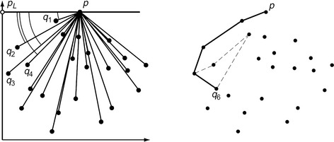
FIGURE 1.20 Left: angles ηi for the vectors defined by q1,q2,q3,q4. Right: a backtrack situation at q6; the dashed edges are removed or not added in Step 4 of the algorithm.
As discussed in Section 1.2.2, simple objects in digital geometry often do not behave like Euclidean objects. Also, for practical purposes, picture size in digital geometry is bounded so that the input data of geometric algorithms have bounded complexity. However, digital geometry is concerned with designing efficient algorithms and has therefore benefited from developments in computational geometry, as we will see in this book. It has also occasionally contributed to computational geometry; here we give just one example.
Definition 1.4
[1001] Let S ![]() B
B ![]() R2. S is called B-convex iff, for all p,q ∈ S, if the straight line segment pq is in B, it is also in S. The B-convex hull of S is the intersection of all B-convex sets that contain S.
R2. S is called B-convex iff, for all p,q ∈ S, if the straight line segment pq is in B, it is also in S. The B-convex hull of S is the intersection of all B-convex sets that contain S.
Figure 1.21 shows two examples of B-convex hulls. If A, B are simple polygons and A is contained in B, it can be shown that the frontier of the B-convex hull of A is the (uniquely determined) minimum-perimeter polygon that is contained in B and that circumscribes A. Such “relative convex hulls” are often used in robotics and computational geometry; they are also useful in digital geometry, as we will see in Chapters 10 and 11.

1.2.10 Fuzzy geometry
When an object in a scene is represented by a set of pixels in a picture, it may not always be obvious which pixels belong to the object. It was suggested in 1970 [825] that “a pictorial object is a fuzzy set which is specified by some membership function defined on all picture points.”
If μ is into {0,1}, it defines an ordinary subset of S, namely Sμ = {x ∈ S:μ(x) = 1};μ is then called the characteristic function of Sμ. Thus an ordinary subset can be regarded as a special type of fuzzy subset.
For any picture P with pixel values in the range {0, …, Gmax}, if we divide the pixel values by Gmax, we obtain a picture P′ in which the pixel values are in the range [0,1], so that they can be regarded as membership values of the pixels in a fuzzy subsetμ of P. For example, μ(p) might represent the degree to which p is associated with some object in the scene. If P is a binary picture, its pixel values are in {0, 1}, and the pixels whose values are 1 define an ordinary subset ![]() of P.
of P.
Figure 1.22 shows a rectangle (on the left) and two “fuzzy rectangles.” In the middle,μ has nonzero membership values only at the pixels of the original rectangle; on the right, some of the pixels outside of the original rectangle also have nonzero membership values.
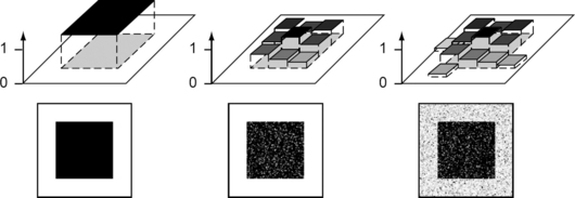
FIGURE 1.22 Lower row: a square in a binary image (left) and two fuzzy squares (middle and right). Upper row: simplified squares with levels in [0,1].
Let μ be a fuzzy subset of S, and let 0 ≤λ ≤ 1. The set μλ = {x ∈ S: μ(x) ≥λ} is called the λ-level set of μ. Evidently μ0 is all of S, and if 0 ≤λ′ ≤λ ≤ 1, we have μλ![]() μ′λ. In later chapters, we will see how geometric properties of subsets of a picture p can be generalized to fuzzy subsets. We will sometimes define a fuzzy subset as having a geometric property (e.g., connectedness, convexity) iff all its level sets have that property.
μ′λ. In later chapters, we will see how geometric properties of subsets of a picture p can be generalized to fuzzy subsets. We will sometimes define a fuzzy subset as having a geometric property (e.g., connectedness, convexity) iff all its level sets have that property.
1.2.11 Integral geometry, isoperimetry, stereology, and tomography
Integral geometry measures properties of a set S in n-dimensional Euclidean space – for example, length L for n = 1; area A, perimeter P, and curvature for n = 2; volume V, surface area S, and (integral of) mean curvature M for n = 3 – by computing integrals of the intersections of S with line segments or convex sets. The values of these integrals are independent of the position and orientation of S; hence they are invariant with respect to the transformations of Euclidean geometry (see Table 1.1 in Section 1.2.2).
The isoperimetric inequality in 2D, which has been known since ancient times, states that, for any planar set that has a well-defined area A and perimeter P, we have the following:
It follows that, among all such sets that have the same perimeter, the disk has the largest area. The expression on the left-hand side of Equation 1.9 is called the shape factor or isoperimetric deficit of the set; it measures how much the set differs from a disk [102]. The first proof of the isoperimetric property of the circle is due to Zenodorus (about 200–140 BC), who is known through the fifth book of the “Mathematic Collection” by Pappus of Alexandria [565].
The study of 3D isoperimetric problems (surface minimizations under volume constraints, possibly with additional boundary or symmetry conditions) has an extensive history involving such famous mathematicians as Euler, the Bernoullis, Gauss, Steiner [1019], and Weierstrass. In 3D, we have the following [391, 746]:
This inequality says that, of all sets with a given surface area, the ball has the largest volume; it has led to studies of the isoperimetric deficit for 3D objects [600]. For bounded convex sets, we also have the following [391, 958]:
For example, a sphere of radius r has mean curvature M = 4πr. See Section 8.3.6 for further formulas involving convex sets.
Buffon’s needle problem is a classic example of a problem in geometric probability that was stated by G.-L. le Comte de Buffon (1707–1788) in 1777 [146]. Draw a set of parallel lines distance d apart in a plane, and toss a needle of length l (0 < l ≤ d) onto the plane. What is the probability that the needle will intersect one or more of the lines? It turns out that this probability is 21/πd; thus needle tossing can be used to estimate the value of π. Stereology uses statistical methods to estimate geometric properties of sets in n-dimensional Euclidean space by measuring intersections of m-dimensional hyperplanes (0 ≤ m <n) with the sets. This characterizes stereology as a field that deals with inverse problems (i.e., determining higher-dimensional sets or functions based on lower-dimensional “observations”).
This book will not usually discuss methods based on integrals, probability, or statistics, but it will be concerned with other methods of estimating properties such as area, perimeter, and so forth, for subsets of a picture. It will also briefly discuss digital tomography in Chapter 14; this is a subfield of discrete tomography,9 which is another example of a field that deals with inverse problems. An early example of a problem studied in discrete tomography is the following: when is a planar convex set uniquely determined by its projections [406]? The case of projections along parallel lines received special attention. We define digital tomography to be the subfield in which the function to be determined or approximated has integer values only and is defined on a finite subset of Z2for some n ≥ 2.
1.2.12 Mathematic morphology
Mathematic morphology (see Chapter 15) makes use of operations based on concepts introduced by J. Steiner (1796–1863) and H. Minkowski (1864–1909) that can be defined on arbitrary vector spaces. For any set A ![]() Rn,
Rn, ![]() = RnA is called the complementary set of A, and
= RnA is called the complementary set of A, and ![]() = {− p: p ∈ A} is called the mirror set of A. A set A
= {− p: p ∈ A} is called the mirror set of A. A set A ![]() Rn is symmetric (with respect to the origin) iff A =
Rn is symmetric (with respect to the origin) iff A = ![]() .
.
The Minkowski sum of A,B ![]() Rn (see Figure 1.23) is as follows:
Rn (see Figure 1.23) is as follows:
The Minkowski difference (actually due to H. Hadwiger [390]; see also [392]) is as follows:

FIGURE 1.23 Examples of the Minkowski sum (left; the original dark-gray set A is contained in the light-gray sum) and the Minkowski difference (right; the original gray set A contains the light-gray difference). In these examples, the set B is the black disk shown in the middle.
For example, ![]() defines a symmetric set with a convex hull that is equal to the Minkowski sum of the convex hulls of A and
defines a symmetric set with a convex hull that is equal to the Minkowski sum of the convex hulls of A and ![]() .
.
In mathematic morphology, (![]() ) is called the erosion of A by B, and (
) is called the erosion of A by B, and (![]() ) is called the dilation of A by B. The opening of A by B is as follows:
) is called the dilation of A by B. The opening of A by B is as follows:
The closing of A by B is as follows:
(For the notation used here, see [969].) These operations have many uses in digital geometry, as we will see in Chapter 15.
1.3 Exercises
1. In a regular grid, in the plane, the grid vertices are connected by grid edges that form simple regular polygons; all of the polygons have the same number m of edges, and every grid vertex is incident with the same number n of grid edges. There are three regular grids in the plane: the orthogonal (square) grid (used in Section 1.1), for which (m, n) = (4,4); the hexagonal grid, for which (m,n) = (6,3); and the triangular grid, for which (m,n) = (3,6). Prove that these are the only possible regular grids in the plane.

2. A center point of one of the regular m-gons that define a regular grid (see Exercise 1) is called a grid point. We can define an xyz-coordinate system for the hexagonal grid; any two of the three coordinates uniquely determine a grid point. Define a test based on the signs of the three coordinates for determining to which sextant (I, II, III, IV, V, VI; see figure) a grid point belongs.

3. Implement the Hilbert scan for pictures of size 2n × 2n (n = 2,3,…, n0).
4. A set S in the Euclidean plane E2 is called polygonally connected iff, for any p,q ∈ S, there is a polygonal arc (p1, p2,…, pn) where p = p1 and q = pn such that the edges of the arc are all contained in S.
(i) Prove that any simple polygon is polygonally connected.
(ii) Consider the four quadrants of the square shown on the left. Specify conditions under which the union of the gray squares or the union of the white squares is polygonally connected. Can you specify conditions under which the union of the gray squares in the upperη rows of the chessboard (on the right) and the union of the white squares in the lower m rows are polygonally connected when 4 ≤ m and n ≤ 8?

5. A set S in the Euclidean plane E2 is called continuously connected iff, for any p,q ∈ S, there is a continuous function f :[0,1] → E2 such that f (0)= p, f (1) = q, and f (x) ∈ S for any real x in the closed interval [0,1]. Give an example of a set S ![]() E2 that is continuously connected but not polygonally connected.
E2 that is continuously connected but not polygonally connected.
6. Specify two metrics d1, d2 on a set S and a subset M ![]() S such that M is unbounded in [S, d1] but bounded in [S, d2].
S such that M is unbounded in [S, d1] but bounded in [S, d2].
7. Prove that property V8 of a vector space follows from properties V0 through V7.
8. Which properties of V0 through V8 of a vector space are satisfied by [Z2, +, ·, R]? (Operations + and· are defined as for [Z2, +, ·, R] in Section 1.2.4.)
9. Let ![]() be the n × n grid (see Equation 1.1), where n ≥ 2, and consider vectors joining two nonidentical points of
be the n × n grid (see Equation 1.1), where n ≥ 2, and consider vectors joining two nonidentical points of ![]() . What is the smallest possible nonzero value of the angleη between two such vectors expressed as a function of n?
. What is the smallest possible nonzero value of the angleη between two such vectors expressed as a function of n?
10. The two figures below appear to be congruent triangles composed of the same four grid polygons. Explain the empty grid square in the figure on the right.

11. Implement the Graham Scan for finite sets of grid points. (Hint: Give arithmetic definitions of “left turns” and “right turns.”)
12. Let S (∏) = P2/4πA (see Equation 1.9) be the shape factor of a simple polygon ∏ with perimeter P and area A. What is S (∏n) if ∏n is a regular n-gon? If κ(n) = |S(∏n) −1|, what is the speed of convergence 1/κ(n) of S to 0 as n→∞?
13. Prove that, among all simple polygons that have the same perimeter and the same number of sides, the regular polygon has the greatest area.
14. In the figure in Exercise 4, let the (closed) gray squares have size 2−n × 2−n; let the large square have size 1 × 1; and let An be the union of the gray squares. (An is illustrated in Exercise 4 for n = 1 and n = 3.) Let Bm = {(x,y):−2 −m ≤ x,y ≤ 2−m} where m ≥ 1. What are A ![]() B, A
B, A ![]() B, AB, and AB where A can be any An(n ≥ 1) and B can be any Bm (m ≥ 1)?
B, AB, and AB where A can be any An(n ≥ 1) and B can be any Bm (m ≥ 1)?
15. Prove that, if n grid points in Z2form a regular n-gon (n > 2), then n = 4. The following figure shows an example on the left.
16. Prove that, if four grid points determine a nonsquare rhombus with angle η (see the figure above on the right), then the quotient η/∏ is irrational. Also prove that, if η is an acute angle of a right triangle with sides that have integer lengths, (called a Pythagorean triangle) then η/π is irrational.
17. Prove that, if all the points in an infinite set are at integer distances from each other, the points must all be collinear.

1.4 Commented Bibliography
Digital geometry is a very lively research area in which many hundreds of journal papers have been published. The study of pictures as mappings defined on rectangular arrays of grid points was initiated in the 1960s and early 1970s in, for example, [286,342,756,881,888,921].
The book chapter [477], Chapter 3 in [992], the books [733, 802,911], and the digital geometry chapter in [891] (all published before 1980), as well as the books [174,430,623,702,805,860,969,1012,1107], define digital geometry as a geometric theory of n-dimensional digital spaces (grid point or grid cell spaces); see also the article [1106].
Digital geometry has its mathematic roots in graph theory and discrete topology; it deals with sets of grid points, which are also studied in the geometry of numbers [732,816], or with cell complexes [9,10], which have also been studied in topology since its beginning [9,10, 659, 660, 820]. Studies of gridding techniques (e.g., by Gauss, Dirichlet, or Jordan [484]) can also be cited as historic context. Digitizations on regular grids are used in many types of numeric calculations.
For the mathematic theory of space-filling curves (also in 3D), see [935]. [996] applies space-filling curves to picture printing. For the Peano curve, see [806]; for the Hilbert curve, see [435].
For more about Euclid, see [564]. Coordinates in geometry are reviewed in [335].10 For Apollonius of Perga, see [24]. For the ancient history of length estimation in mathematics (e.g., the work of Archimedes and Liu Hui on the estimation of π), see [1083]. The error measure in Equation 1.8 is discussed in [543].
For the history of graph theory, see [89]. [299,394, 789, 1145] are monographs about combinatorial geometry, and [97, 300, 823] are textbooks about computational geometry. For Graham’s Scan, see [375].
For integral geometry and stereology, see [17, 858]. “Discrete integral geometry,” following [1107, 1108], will be treated in Chapters 4 and 5. For discrete tomography, see [380, 431]. For the Minkowski sum, see [731]; for the Minkowski difference, see [390].
For early work on fuzzy convexity, see [670, 1157], and for early work on fuzzy topology, see [892]. “Fuzzy shape transforms” were introduced in [644]. The review [900] discusses a variety of fuzzy geometric properties that had been studied by 1984.
A geometric model of the panoramic picture acquisition process (see Figure 1.3) is discussed in [447]. There are many papers about hexagonal grids (Exercises 1 and 2); see, for example, [132] for properties and advantages of such grids, and see also [68, 105, 1015]. For semiregular grids, see [106]. Exercise 13 is due to Zenodorus [565]. For Exercise 14, see [961]. Exercise 15 follows from a general theorem in [389]: if 0 < η < π/2 and the number cos η is rational, then either η = π/3 or η/π is irrational. For Exercise 16, see [307].
1These are the most common types of two-valued pictures that are used in picture analysis, but using the values + 1 and − 1 may be convenient in some algorithms. If there are more than two values, we call the picture multivalued
2Read “if and only if”; acronym proposed by P.R. Halmos.
3A mathematic paradox (antinomy) is characterized by the deduction of a contradiction within a theory. The existence of statements in digital topology that do not resemble statements in Euclidean topology is not a mathematic paradox.
4See pages 26–27 in the English translation of [264].
5Two sets are called incident if one of them contains the other. In all of these geometries, incidences between sets (e.g., between points and lines) are invariant.
6In an 1861 publication, Listing writes that “topologische Eigenschaften (solche sind), die sich nicht auf die Quantität und das Maass der Ausdehnung, sondern auf den Modus der Anordnung und Lage beziehen.” (Translation: Topologic properties are those that are related not to quantity or content but to spatial order and position.) Because Listing was a student and then a close friend of C.F. Gauss, Listing’s interest in the subject may have followed the advice or example of Gauss himself.
7This will be defined later (see Chapter 6) as a connected set that has a trivial fundamental group. Informally, a simply connected set in 3D space is connected and has no cavities or tunnels. In general, a “cut” creates a (doubly oriented) simple arc, simple curve, or simply connected face. Removing a single point from a hollow sphere transforms it into a simply connected object; this is the limiting case of a circular cut that has radius 0.
8In a Cartesian coordinate system, a line is called isothetic iff it is parallel to a coordinate axis; a plane is called isothetic iff it is parallel to a coordinate plane. An isothetic polygon has only isothetic edges, and an isothetic polyhedron has only isothetic faces. A polygon is called a grid polygon and a polyhedron is called a grid polyhedron if their vertices are grid points. In this book, we will often deal with isothetic grid polygons and polyhedra.
9This was the name of the first meeting on the subject in 1994, which was organized by L. Shepp. Tomography is concerned with determining or approximating a function defined on a discrete or continuous set given a collection of weighted sums or weighted integrals of the function over subsets of its domain.
10Descartes’ friends pressured him into publishing some of his work. In 1637, his first scientific book was published in Leyden [264]. Descartes’ method consisted of doubting all accepted knowledge (a mortal sin for orthodox thinkers), basing all thinking on clear self-evident truths, and using logical reasoning (based on mathematics) to build up a system of ideas. He explained the advantages of the top-down approach to large and difficult problems, breaking them into smaller problems in such a way that the solutions to the smaller problems could be combined to solve the large problem. The part of his book entitled La Géomètrie united algebra and geometry and introduced algebraic notation that was so much better than anything previous that it has remained almost unchanged since 1637. La Géomètrie is the earliest book that a modern mathematician can read without having to learn obsolete notation and terminology; it is generally regarded as the foundation of modern mathematics.