
Grids and Digitization
This chapter begins by defining the 2D and 3D grid point and grid cell adjacency models as well as a more refined cell model called the grid (cell) incidence model, which combines cells of different dimensionalities. It then discusses connectedness (the reflexive and transitive closure of adjacency) and algorithms for identifying (‘labeling”) connected components. It also discusses digitization models, including the classic Gauss, Jordan, and grid intersection models, and defines a ‘domain” model that generalizes all of them.
Measurements made on digital pictures can only approximate the measurements that might ideally have been made on real objects or real pictures. Digital geometry deals with the computation of geometric measurements (or properties or relations) from digital pictures and with the study of how well these measurements approximate the corresponding ideal measurements on the real objects or pictures. This chapter introduces a methodology called multigrid convergence for comparing ideal and approximate measurements.
2.1 The Grid Pointand Grid Cell Modesls
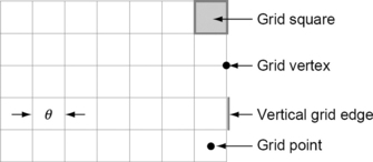
Figure 2.1 illustrates a portion of a 2D grid with grid constant θ (see Section 1.2.1). We will first assume that θ = 1, and we will discuss θ as a variable later in this section.
2.1.1 Grid points and grid cells
In 2D, the grid point set is Z2, and, in 3D, the grid point set is Z3. A grid vertex is shifted by (0·5,0·5) with respect to a grid point in 2D and by (0·5, 0·5, 0·5) in 3D.1 A pair of adjacent grid vertices (i.e., vertices at Euclidean distance 1 from each other)defines a grid edge. A grid square is defined by four grid edges that form a square, and a grid cube in 3D is defined by six grid squares that form a cube.
We specify grid points, vertices, edges, squares, and cubes in terms of Cartesian coordinates. In 2D, the set of positions of the grid vertices is as follows:
A grid edge2 connects a pair of adjacent grid vertices:
A grid square is defined by a quadruple of grid edges in which successive edges (modulo 4) share a vertex.
In 3D, the positions of grid vertices, grid edges, grid squares, and grid cubes are specified similarly.
In both 2D and 3D, the sets of grid vertices and grid points are congruent This supports the use in this book of the same planar or spatial grid for 2D or 3D pictures when we use either the grid cell or grid point model.
The dimensionalities 3, 2,1, and 0 of grid cubes, grid squares, grid edges, and grid vertices suggest an alternative terminology:
In this terminology, a 2D grid point is the center point of a 2-cell (see Figures 2.2 and 2.3), and a 3D grid point is the center point of a 3-cell. C(i)2 will denote the set of all i-cells in the plane (i = 0,1,2), and C(i)2 will denote the set of all i-cells in 3D space (i = 0,1,2,3). We also define the following:


(The symbol ![]() is often used in the mathematic literature for the set of complex numbers, but this book will make no use of complex numbers, so there is no conflict when using
is often used in the mathematic literature for the set of complex numbers, but this book will make no use of complex numbers, so there is no conflict when using ![]() to denote sets of cells.)
to denote sets of cells.)
We now define the two basic grid models that will be used throughout this book:
• In the grid point model, a 2D grid G is either the infinite grid Z2 or an m × n rectangular subarray of Z2; see Gm,n in Equation 1.1. Similarly, a 3D grid is either Z3 or an l × m × n cuboidal subarray of Z3.
• In the grid cell model, a 2D grid G is either C2 or an m × n ‘block” of 2-cells whose union ∪G is a rectangular region of the Euclidean plane E2; see Gm,n in Equation 1.2. Similarly, a 3D grid is either C3 or an l × m × n set of 3-cells whose union is a cuboid in Euclidean space E3.
These grids can also be defined for a grid constant θ different from 1, but θ = 1 is the default value throughout this book. Grid cells or grid points are the basic elements used in digital geometry. A pixel is either a 2-cell (grid square) or a grid point (the center of a 2-cell); see Figure 2.2. A voxel is either a 3-cell (grid cube) or a grid point (the center of a 3-cell). The formulation of a definition or algorithm may sometimes be more convenient when one or the other model is used.
A grid line in 2D is incident with two different grid points whose x- or y-coordinates are the same. The 2D grid Z2 can be regarded as a subset of the 3D grid Z3 by adding a third coordinate z = 0 to every 2D grid point. In 3D, a grid plane is incident with two orthogonal grid lines. It follows that all of the grid points of a grid plane have the same x-, y-, or z-coordinate. A grid line in 3D is a set of points, two with coordinates that are constant in Z, whereas the third is a variable in R. Grid lines intersect at grid points in either 2D or 3D.
2.1.2 Variable grid resolution
The grid constant θ is the distance between neighboring grid lines. Grid resolution is the inverse of the grid constant. It refers to the number of grid elements per unit of distance without specifying the physical size of the unit. We will use an integer parameter h gt; 0 to denote grid resolution. In a grid with resolution h = 1, we can have either one grid point in a unit or two grid points as endpoints of a unit. In general, the maximum number of grid points per unit is h + 1.3
The parameters h and θ are useful when discussing the possible effects of improvements in geometric or picture resolution. They are especially relevant in theoretic studies of the convergence behavior of algorithms under refinement of grid resolution (i.e., decrease of the grid constant).
Let Zh = {i/h : i Z}; then is the set of all 2D grid points in a grid of resolution h gt; 0, and ![]() is the set of all such 3D grid points. We similarly use the notation
is the set of all such 3D grid points. We similarly use the notation
2.1.3 Adjacencies in 2D grids
In other words, two 2-cells c1 and c2 are 1-adjacent iff they are not identical but they share a grid edge. Let pi be the center of ci (i = 1,2); then c1 and c2 are 1-adjacent iff p1 and p2 are 4-adjacent
We have defined relations A1 of 1-adjacency and A4 of 4-adjacency for the grid cell and grid point models. In general, we write pRq or (x,y)∈ R iff p,q are in relation R. In this notation, we have c1A1c2 iff {c1,c2} ∈ A1, iff c1 and c2 are 1-adjacent, and p1A4p2 iff {p1,p2} ∈A4 iff p1,p2 are 4-adjacent. The relation A1 (A4) is symmetric and irreflexive.
In other words, two 2-cells c1 and c2 are 0-adjacent iff they are not identical but share (at least) a grid vertex. Again, let pi be the center of ci (i = 1,2); then c1 and c2 are 0-adjacent iff p1 and p2 are 8-adjacent. The relation A0 (A8) is symmetric and irreflexive.Figure 2.4 illustrates relations A0, A, A4, and A8 on a square grid.

FIGURE 2.4 Consecutive sequences of adjacent pixels for adjacency relations A1and A4 (on the left), A0 and A8 (on the right).
Adjacent 2-cells are transformed into adjacent grid points by mapping the 2-cells onto their center points, and adjacent grid points are transformed into adjacent 2-cells by mapping the grid points into the 2-cells that have them as center points. The existence of this one-to-one mapping gives us the following:
(In general, let R1 be a relation on a set S1 and R2 a relation on a set S2. The structures [S1, R1] and [S2, R2] are called isomorphic iff there exists a one-to-one mapping f from S1 onto S2 such that pR1q iff f (p)R2f (q) for all p,q ∈ S1. The mapping is called an isomorphism.)
For the relations A1 and A4 on C2 (Z2), the number of pixels (grid points or grid cells) adjacent to a pixel is always 4. For A0 and A8, it is always 8; however, for adjacency relations defined on pictures, the number can vary.
Adjacencies between pixels in multilevel pictures are defined by locations and pixel values. To start with, let us consider the values alone. Let P be a picturedefined on the grid G in which pixel p has value P (p) in {0,1,…,Gmax}. We say that two pixels p and q are P-equivalent iff P(p) = P(q). Let Mu be the set of all qg such that P(q)= u. If there exists pg such that u = P(p), Mu is an equivalence class with respect to the relation of P-equivalence on G (in brief, a P-equivalence class).
These P-equivalence classes are defined only by pixel values, not by locations. Each P-equivalence class splits into components, depending on the adjacency relation used for the pixels. For example, we can define p and q to be P-adjacent if they are 8-adjacent (or 0-adjacent) and P-equivalent. The number of pixels P-adjacent to p can then vary between 0 and 8. Using 8-adjacency uniformly for all values u may lead to situations such as the one illustrated in Figure 1.9.d (If there are more than two values, we cannot use 4-connectedness for one value and 8-connectedness for the other as proposed in Section 1.1.4 for binary pictures.)
More generally, we can model ‘uncertainties” in picture values by assuming that we are given a similarity relation σ (a reflexive and symmetric relation) on V × V, where V = {0,1,…,Gmax}. (For example,σ2 is the similarity relation in which uσ2v iff |u – v|≤ 2.) Define two pixels p,q to be σ,α)-adjacent iff pA αq and P(p)σP(q). The relation of (σ,α)-adjacency is symmetric and irreflexive. Note that p may have no (σ,α)-adjacent pixels if P(p) is not σ-similar to the value of any of the pixels that are α-adjacent to p.
In the remainder of this section, we describe a method of defining adjacencies in a 2D multivalued picture P, which we call switch adjacency (or s-adjacency) and denote with As. Switch adjacency allows us to avoid topologic conflicts (see Section 1.1.4 about binary pictures).
Pairs of 4-adjacent pixels are always regarded as s-adjacent; in other words, As ⊇ A4. In addition, in each 2 × 2 block of pixels, we call exactly one of the two diagonally adjacent pairs s-adjacent. We can think of the 2 × 2 block as a switch that can be in either of the two diagonal positions (see Figure 2.5); the position of the switch determines which diagonally adjacent pair of pixels in the block is regarded as s-adjacent. The states of the switches in P can be specified by a binary picture S (a ‘switch state matrix”) that has pixels that correspond to the lower left-hand corners of the 2 × 2 blocks of pixels in P. A pixel of S has value 1 iff the switch in the corresponding 2 × 2 block of P is to the left (in the main diagonal position) and value 0 iff that switch is to the right (in the other diagonal position).
We can define specific s-adjacency relations in many ways. The switch position in a block can depend on the position of the block (i.e., on the coordinates of its lower left-hand corner) and not on the values of the pixels in the block. For example, S can be the binary picture in which pixel (x,y) has value 1 if y is odd and 0 if y is even. (In this case, two pixels are s-adjacent iff their hexagonal distance dh is 1;see the leftmost image of Figure 2.7, and see Section 3.2.3 about metric dh.) It is more ‘natural” to let the diagonal s-adjacencies depend on the pixel values. Let the difference between the values of one pair of diagonally adjacent pixels in a 2 × 2 block be d1 and the difference between the values of the other pair be d2; if d1 d2, we call the first pair s-adjacent; if d2 d1, we call the second pair s-adjacent. This determines all of the s-adjacencies, except in flip-flop cases, where d1 = d2; in such a case, the switch can be in either position. In real pictures, flip-flop cases are rare (see Figure 2.6); there are typically less than 0.5% of such cases in a grayscale picture and less than 0.2% in a color picture (see Figure 2.8 for four grayscale examples).


FIGURE 2.7 Two examples of (regular) s-adjacencies where switch positions depend only on block positions (left and middle), and an irregular s-adjacency relation (right).

FIGURE 2.8 These pictures are of size 2014 × 1426 (so that they contain 2,872,964 pixels) and have Gmax = 255. The picture at the upper left position has only 14,359 flip-flop cases (i.e., 0.5% of the pixels). In the pictures in the upper right, lower left, and lower right positions, the percentages of flip-flop cases are 0.38%, 0.38%, and 0.22%, respectively.
Evidently the s-adjacency relation is symmetric and irreflexive. The number of pixels s-adjacent to p can be anywhere between 4 (the pixels 4-adjacent to p) and 8 (up to four additional diagonal adjacencies).
In general, we can use a Set Switches procedure to define a switch state matrix S. The procedure can analyze larger neighborhoods of a pixel to determine the state of its switch. This analysis can be based on templates such as those shown in Figure 2.9 in which the state of the switch in the lower 2 × 2 block is also used in the upper 2 × 2 block. S can even be generated randomly (using a random number generator) or using a function of the pixel coordinates (e.g., a pseudorandom function, to avoid bias).

2.1.4 Adjacencies in 3D grids
The definitions of 1-adjacency and 0-adjacency of 2-cells (Definitions 2.2 and 2.3) can also be used in 3D, and we can also define the 0-adjacency of 1-cells. However, ourmain interest is in adjacencies between 3-cells or 3D grid points. Let de be the Euclidean metric (see Section 1.2.1).
Definition 2.4
Two 3-cells c1 and c2 are called α-adjacent iff c1 ≠ c2 and the intersection c1 ∩ c2 contains an α-cell (α ∈ {0,1,2}). Two 3D grid points p1 = (x1,y1,z1) and p2 = (x2,y2,z2) are called 6-adjacent iff 0 de(p1,p2) ≤ 1, 18-adjacent iff 0 de(p1,p2) ≤ ![]() , and 26-adjacent iff 0 de(p1,p2) ≤
, and 26-adjacent iff 0 de(p1,p2) ≤ ![]()
Let c1 and c2 be 3-cells and let pi be the center of ci (i = 1, 2). Then c1 and c2 are 0-adjacent iff p1 and p2 are 26-adjacent iff c1 and c2 are not identical but share a grid vertex; c1 and c2 are 1-adjacent iff p1 and p2 are 18-adjacent iff c1 and c2 are not identical but share a grid edge; and c1 and c2 are 2-adjacent iff p1 and p2 are 6-adjacent iff c1 and c2 are not identical but share a grid square (see Figure 2.10).

FIGURE 2.10 Left: two α-adjacent 3-cells (α = 0,1,2). Middle: two α-adjacent 3-cells (α = 0,1). Right: two 0-adjacent 3-cells.
This defines symmetric and irreflexive relations Aα, where α = 0,1,2 for the grid cell model and α = 6, 18, 26 for the grid point model. The parameter α denotes the dimension of the intersection of the grid cells in the first case and the number of adjacent grid points in the second case.
Data-dependent types of adjacencies (see Section 2.1.3) can also be generalized to 3D grids. We can now define the 2D and 3D grid point and grid cell adjacency models:
• A 2D (3D) grid point adjacency model combines the grid point model with an adjacency relation defined between 2D (3D) grid points.
• A 2D (3D) grid cell adjacency model combines the grid cell model with an adjacency relation defined between grid squares (grid cubes).
Both 2D and 3D grid point and grid cell adjacency models are called α-adjacency grids; the value of α determines whether we use a grid point model (α > 4) or a grid cell model (α ≤ 3). In Section 1.1.4, we briefly mentioned a dual use of adjacencies for 2D binary pictures P:α1-adjacency for ![]() and α2-adjacency for
and α2-adjacency for ![]() ; in this case we speak about (α1,α2)-adjacency grids.
; in this case we speak about (α1,α2)-adjacency grids.
Let A be a symmetric and irreflexive adjacency relation on a set S. A(p) = {q : q![]() S ∧ qAp} is called the adjacency set of p∈S. For example, for relation A4 on grid points, we have the following,
S ∧ qAp} is called the adjacency set of p∈S. For example, for relation A4 on grid points, we have the following,
provided all four of these grid points are also contained in the grid Gm,n.
N(p) = A(p)∪{p} is called the (smallest nontrivial) neighborhood of p ∈ S defined by adjacency relation A. N defines a symmetric and reflexive relation qNpon S.p ∈ S is never in A(p) but is always in N(p). Figure 2.11 shows A1 (A4) and N1 (N4) for the 2D grid cell and grid point models. Analogous drawings for A0 (A8) and N0(p) (N8(p)) would also contain the grid cells or grid points in the four corners.

2.1.5 Grid cell incidence
Two sets are called incident iff one of them contains the other (i.e., any set is incident with itself). For example, a 3D grid vertex (0-cell) is incident with six grid edges (1-cells); a grid square (2-cell) is incident with four grid edges; and a grid cube (3-cell) is incident with 12 grid edges.
Figure 2.12 shows four ways of representing a 2D grid. In the grid cell model, we can use only 2-cells (upper right), or we can also use 0- and 1-cells (lower right). In the first case, we can use 0- or 1-adjacency to define a grid cell adjacency model, and, in the second case, we use the incidence relations between all of the cells to define the 2D grid cell incidence model.

FIGURE 2.12 Four ways of representing a 2D grid. Adjacency or incidence relations can be defined on the grid points or grid cells.
There exists a grid point adjacency (incidence) model that is isomorphic to any of these grid cell adjacency (incidence) models. For grid points, we usually use only an adjacency model; however, for completeness, we mention that a grid point incidence model can be defined by adding isothetic edges between grid points—and “loops” consisting of quadruples of such edges—to the set of grid points. This refined model is isomorphic to the grid cell incidence model. In the correspondence between the models, a grid point p is the center of a 2-cell, an isothetic edge connecting p with another grid point intersects a 1-cell, and a loop of four such edges has a 0-cell as its center. The dimensions of the elements in the grid point incidence model are defined by the dimensions of the corresponding cells; for example, a loop is zero-dimensional.
Analogously, there are four types of models for 3D grids: (1) grid point and (2) grid cell adjacency models (see Section 2.1.4); (3) a grid cell incidence model that includes 0-, 1-, and 2-cells in addition to 3-cells (and again, for completeness, (4) the grid point model allows a structure that is isomorphic to the grid cell incidence model in which a grid point corresponds to a 3-cell [in which it is the center]); an isothetic edge between two grid points corresponds to a 2-cell (which it intersects at its center point), a loop of four isothetic edges corresponds to a 1-cell (where the loop defines a square having the 1-cell at its center), and 12 such edges forming a cube correspond to a 0-cell (at the center of the cube).
The 2D and 3D grid cell incidence models are called (2D or 3D) incidence grids.
This definition leads to a recursive test for completeness: start with the 3-cells, then check the 2-cells between them, then check the 1-cells that are incident only with 2- or 3-cells already known to be in M, and so on.
The geometric representation of the 2D incidence grid used in this book is illustrated in Figure 2.13: 0-cells are small squares (representing grid vertices);1-cells are thin rectangles (representing grid edges); and 2-cells are large squares.4In 3D, we use a similar representation, with small cubes as 0-cells, large cubes as 3-cells, and elongated (flat) cuboids as 1-cells (2-cells); see Figure 2.14. Despite these geometric representations, an i-cell is still considered to be of (abstract) dimension i.


2.2 Connected Components
The concept of connectedness defined in Section 1.1.4 applies to any of the adjacency relations defined in Section 2.1 for 2D or 3D grids. We recall that the reflexive and transitive closure of an adjacency relation is called a connectedness relation. In other words, any element of the grid is connected to itself, and two elements p and q of the grid are connected iff there exists a sequence of elements (p0,…,pn) where n > 0 such that p0 = p, pn = q, and pi+1 is adjacent to pi (0 ≤ i < n).
2.2.1 Connectedness and components
Let G be an adjacency grid. A sequenceρ = (p0,…,pn) of pixels or voxels, where p0 = p, pn = q, and pi+1 is adjacent to pi (0 ≤ i ≤ n − 1), is called a path of length n from p to q, and p and q are called the endpixels or endvoxels ofρ. The elements p and q are called connected if there is a path from p to q. In particular, for α-adjacency (α {0, 1, 2, 3, 4, 6, 8, 18, 26}), we use the terms ‘α-path” and ‘α-connected.”
Figure 2.15 shows a 1-path of 2-cells in the grid cell model and the corresponding 4-path in the grid point model. Figure 2.16 shows a 2-path of 3-cells in the grid cell model and the corresponding 6-path in the grid point model.

FIGURE 2.15 A 1-path in the grid cell model (left) that corresponds with a 4-path in the grid point model (right).
FIGURE 2.16 A 2-path in the grid cell model (left) that corresponds with a 6-path in the grid point model (right).
Let M be a finite subset of G. A maximal connected set of pixels or voxels of M is called a component of M. Evidently p, q M are in the same component of M iff there is a path completely contained in M that has p and q as endpixels (endvoxels).
Let Gm,n be an m × n grid. (Similar remarks apply to an l × m × n grid Gl,m,n) Gm,n can be extended into the infinite discrete plane (Z2 in the case of the grid point model; ![]() in the case of the grid cell model). Let M be a subset of Gm,n; thus the complement
in the case of the grid cell model). Let M be a subset of Gm,n; thus the complement ![]() of M contains the complement
of M contains the complement ![]() m,n of G. The (infinite) set of pixels of M that are connected to pixels of Gm,n is called the background component of M. Any other pixel of
m,n of G. The (infinite) set of pixels of M that are connected to pixels of Gm,n is called the background component of M. Any other pixel of ![]() belongs to a finite component of
belongs to a finite component of ![]() .
.
Let P be a picture defined on G. The P-equivalence classes define subsets of G. Components of these classes are often of interest, as we will see in later chapters. Figure 2.17 illustrates the components defined by these classes in a 5-valued picture using 1-adjacency in the grid cell model. Class 5 consists of six 1-components (also defining two complementary 1-components, one of which belongs to the background 1-component of class 5); class 4 consists of five 1-components (both complementary 1-components belong to the background 1-component of class 4); class 3 consists of four 1-components (one complementary 1-component); class 2 consists of four 1-components (two complementary 1-components, both belonging to the background 1-component of class 2); and class 1 consists of three 1-components.

FIGURE 2.17 A picture that has five P-equivalence classes; the numbers on the right are used to refer to these classes in the text.
In the 2D or 3D incidence grid, two cells c1 and c2 are called k-adjacent iff they are not identical and there is a k-cell c (c ≠ c1 and c ≠ c2) that is incident with both c1 and c2
Figure 2.18 shows examples of paths for these adjacency relations. This definition generalizes the concepts of 1-adjacency (see Definition 2.2) and 0-adjacency (see Definition 2.3) between 2-cells or of α-adjacency (0 ≤α ≤ 2) between 3-cells (see Definition 2.4). Connectedness and components in 2D or 3D incidence grids can be defined using these adjacency relations.

FIGURE 2.18 Top row: a 1-path of 2-cells (left) and a 0-path of 1-cells (right) in the 2D incidence grid. Bottom row: a 2-path of 3-cells (left), a 1-path of 2-cells (middle), and a 0-path of 1-cells (right) in the 3D incidence grid.
The following two propositions show that for pictures defined on an incidence grid, cells can be assigned to P-equivalence classes in such a way that the componentsof the classes are complete. We give the proof for the 2D grid only; the 3D generalization is straightforward.
Figure 2.19 shows an example of such an assignment for the picture P shown in Figure 2.17. Note that we do not need an extended data structure to represent P on an incidence grid; all of the assignments of 0- or 1-cells are determined by the order of the picture values.

2.2.2 Counting connected sets
A finite connected subset of the 1-adjacency grid[![]() ] is called a polyomino. (Polyominoes illustrate the combinatorial complexity of finite sets of pixels; see Chapters 13 and 14 about polyominoes in the context of digital convexity and digital tomography.) If it consists of exactly n grid squares, it is called an n-omino.
] is called a polyomino. (Polyominoes illustrate the combinatorial complexity of finite sets of pixels; see Chapters 13 and 14 about polyominoes in the context of digital convexity and digital tomography.) If it consists of exactly n grid squares, it is called an n-omino.
Equivalence classes of polyominoes can be defined with respect to geometric transformations that map the grid into itself. Such transformations include (see also Section 14.4) translations by vectors (i,j), i, jZ∈ rotations around the origin by 90°, 180°, or 270° and reflections in the x- or y-axis.
Two polyominoes are called translation-equivalent if there is a translation that maps one of them into the other. A translation-equivalence class of polyominoes is called a fixed polyomino. An equivalence class of polyominoes with respect to translations and rotations is called a chiral polyomino; an equivalence class of polyominoes under translations, rotations, and reflections (a congruence class) is called a free polyomino.5
Figure 2.20 shows the 12 free 5-ominoes. Figure 2.21 shows the 369 free 8-ominoes (the 8-ominoes that contain a hole are positioned in the center of the figure; the filled dots indicate 8-ominoes that contain at least one 2 × 2 block).
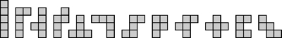

FIGURE 2.21 The 369 free 8-ominoes [368]
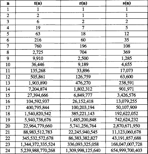
The numbers of fixed n-ominoes, chiral n-ominoes, and free n-ominoes are denoted by t(n), r(n), and s(n), respectively. It is not hard to show the following:
There are no simple formulas for these functions, but the following has been demonstrated [371]:
Table 2.1 shows the values of t(n),r(n), and s(n) for 1 ≤ n ≤ 24. The calculation of these functions is a topic in the theory of polyominoes. Redelmeier’s algorithm [839] for calculating them has exponential time complexity; no algorithm is yet known that has subexponential time complexity. An algorithm for generating polyominoes would also be of interest; it could be used to generate data sets for testing algorithms in digital geometry.
2.2.3 Component labeling
The following task arises frequently in picture analysis and computer graphics; it is known as labeling, filling, or region detection. Let P be a 2D multivalued picture defined on a finite adjacency or incidence grid G, and let the P-equivalence classes have a total of k components. We regard the (infinite) complement of G as consisting of pixels that all have the same value, so they belong to one of the components. The task is to assign k labels (e.g., integers) to the pixels of P in such a way that all ofthe pixels in each component have the same label and pixels in different components have different labels. To keep P unaltered, we can put the labels into an array of the same size as P.
A simple method of labeling components is as follows. Scan the picture until a pixel p is found that has not yet been labeled. Suppose P(p)=u and that labels L1,…,Lk−1 have already been used. Choose a new label Lk, and call the procedure FILL(p, u,Lk) (see Algorithm 2.1). (Note that the adjacency set A(r) may depend on u [e.g., if we use 1-adjacency for 1s and 0-adjacency for 0s].) After labeling the component that contains p, continue scanning the picture until all of the pixels have been labeled.6Figure 2.22 shows the order of the pixel visits (assuming the ordershown on the right is used for visiting 1-adjacent pixels) when this algorithm is used to label the white pixels of the picture in Figure 2.23.

FIGURE 2.22 The numbers show the order in which the pixels are labeled, assuming a standard scan. The diagram on the right shows the order in which 1-adjacent pixels are visited.

FIGURE 2.23 Let P be the binary picture shown on the left. If we use (1,0)-adjacency and the standard scan and assume that the infinite background component is black, the algorithm produces the label assignments shown on the right and the equivalence table shown in Table 2.2.
The Rosenfeld-Pfaltz labeling algorithm [921] labels all of the components of P in two scans of P (see Section 1.1.3); see Algorithm 2.2 In the first scan, we propagate smallest labels, and, whenever labels merge, we note this fact in a table of equivalent pairs of labels. In the second scan, we replace each label with a representative of its equivalence class. This algorithm replaces the use of a stack (of size mn) in procedure FILL with the use of an equivalence table; its run time can be compared with that of the simple depth-first search procedure for given classes of pictures. It also provides an illustration of the cases that can occur during component labeling.
As an example of the operation of this algorithm, consider the binary picture shown in Figure 2.23. In the label propagation step of the algorithm, we use 1-adjacency for white pixels and 0-adjacency for black pixels. At the end of the first scan (a standard scan), we have the equivalence table shown in Table 2.2. Label A is also the label of all of the pixels of the background component. Note that some equivalences are detected more than once.

The equivalences between pairs of the 20 labels A,…,T are shown in Figure 2.24. We will use the smallest label in each equivalence class as the pivot of that class.

To find the pivots, we scan the labels in order, smallest first. Any label that is equivalent to A has pivot A and can be marked and replaced with A. We next examine the smallest label that has not yet been marked; this label must be the pivot of its equivalence class so that all of the labels equivalent to it can be marked and replaced with it. This process is repeated until all of the labels have been marked.7The pivots in our example are shown in Table 2.3.
A binary picture of size m × n in which 0s and 1s alternate (‘a chessboard”) requires O(mn) labels. An a priori threshold on the number of labels can be used to limit the size of the equivalence table. However, memory limitations are no longer an issue, which they were in 1966, when the algorithm was first published.
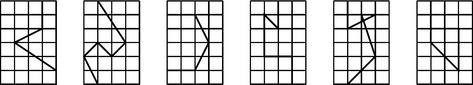
The nontriviality of connected component labeling is illustrated in Figure 2.25. In one of these binary pictures, the black pixels are connected, and in the other one, there are two 4-components of black pixels; can you tell which is which?
FIGURE 2.25 In which of these pictures are the black pixels connected [631].
2.3 Digitization Models
We use mathematically defined methods of digitization to create digital pictures and to compare results obtained by analyzing these pictures with correspondingresults in Euclidean or similarity geometry (see Section 1.2.2). In this section, we describe three digitization methods: Gauss digitization and grid-intersection digitization, which were originally proposed for 2D, and Jordan digitization, which was defined more than a century ago for 3D. We generalize these methods to allow variable grid resolution, and we extend the Gauss and grid-intersection models to 3D and the Jordan model to 2D. We define these digitization methods for the grid cell model, but they can also be used with the grid point model by representing cells with their centers. We briefly discuss relationships among these digitizations, and we conclude by defining a general class of digitization methods that has all of these methods as special cases.
2.3.1 Gauss digitization
C.F. Gauss (1777–1855) studied the measurement of the area of a planar set S ⊂ R2 by counting the grid points (i,j)∈Z2 contained in S. This approach suggests the following:
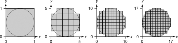
Figure 2.26 shows the Gauss digitizations G(D) of four disks D of different diameters (measured in grid units). (The results would be the same if the disks all had unit diameter and were digitized on grids of different resolutions. The Gauss digitization of S on a grid of resolution h will be denoted by Gh(S).) G(D) is an isothetic polygon that has 12 vertices for diameter 5, 20 vertices for diameter 10, and 36 vertices for diameter 17. Note that the number of vertices is always a multiple of 4, because a disk that is centered at a grid point has a symmetric Gauss digitization.
Obviously, different sets can have identical Gauss digitizations. Figure 2.27 shows the Gauss digitization of a simple polygon Π with area 102,742.5 and perimeter 4,040.796,631… drawn on a 512 × 512 grid. On the upper left, each grid squarecontains 64 × 64 squares of the original 512 × 512 grid; in the upper middle, 32 × 32; and so on.
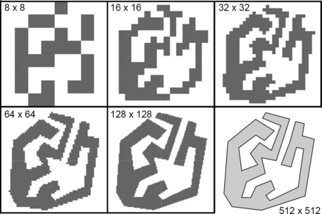
FIGURE 2.27 Gauss digitization of a simple polygon using grids of sizes from 8 × 8 (upper left) to 128 × 128 (lower middle). The original polygon was drawn on a grid of size 512 × 512 (lower right).
Figure 2.28 shows the relative deviations of the area and perimeter of Gh (Π) from those of Π when Π is digitized on a 2n × 2n grid (i.e., h = 2n). The relative deviation is the absolute difference between the property values for Gh (Π) and Π divided by the property value for Π. See Chapter 4 for an in-depth discussion about perimeter estimation; the perimeter of Gh(Π) (i.e., the number of 1-cells on its frontier) is not a good estimate of the perimeter of Π.

FIGURE 2.28 Relative deviations of area and perimeter for the digitized polygon in Figure 2.27.
Gauss digitization is defined analogously in 3D. If S ⊂ R3, the Gauss digitization Gh(S) is the union of all of the 3-cells (in a grid of resolution h gt; 0) with center points in S.
2.3.2 Jordan digitization
Let S ⊂ R3 and h gt; 0. The magnification of S by factor h is denoted by h. S. In terms of multiplication of vectors by a scalar (see Section 1.2.12), we have the following:
This magnification leaves the origin (0,0,0) fixed; other points of R3 could also be chosen as fixed points.
C. Jordan (1838–1922) [484] used grids to estimate the volumes of subsets of R3. Let S ⊂ R3 be contained in the union of finitely many 3-cells. Magnify S by factor h with respect to an arbitrary fixed point p R3; this transforms S into ![]() . Let
. Let ![]() (S) be the number of 3-cells completely contained in
(S) be the number of 3-cells completely contained in ![]() and
and ![]() the number of 3-cells that have nonempty intersections with
the number of 3-cells that have nonempty intersections with ![]() . Then
. Then ![]() and
and ![]() converge to limits L(S) and U(S), respectively, as h goes to infinity; these limits are the same for any p [484]. Jordan called L(S) the inner volume and U(S) the outer volume of S or the volume V(S) of S if L(S) = U(S).
converge to limits L(S) and U(S), respectively, as h goes to infinity; these limits are the same for any p [484]. Jordan called L(S) the inner volume and U(S) the outer volume of S or the volume V(S) of S if L(S) = U(S).
We use Jordan’s digitization model for subsets of the plane as well as of 3D space:
Definition 2.8
Let S be a nonempty subset of R2. Let ![]() (S) be the union of all 2-cells (for grid resolution h gt;0) that are completely contained in S, and let
(S) be the union of all 2-cells (for grid resolution h gt;0) that are completely contained in S, and let ![]() (S) be the union of all such 2-cells that have nonempty intersections with S.
(S) be the union of all such 2-cells that have nonempty intersections with S. ![]() (S) is called the inner Jordan digitization of S and
(S) is called the inner Jordan digitization of S and ![]() (S) the outer Jordan digitization of S. For S ⊆ R3, we use 3-cells instead of 2-cells. For brevity, we denote
(S) the outer Jordan digitization of S. For S ⊆ R3, we use 3-cells instead of 2-cells. For brevity, we denote ![]() and
and ![]() with
with ![]() and
and ![]() respectively.
respectively.
Outer Jordan digitization is also called super-cover digitization [209]. (Inner Jordan digitization will be further specified in Section 3.2.5 by one additional [topologic] constraint that is still missing in the above definition.) Figure 2.29 shows a 2D example in which S is a circle of radius n (in grid units) for n = 4 (left), n = 8 (middle), and n = 16 (right). If the frontier of a nonempty set S ⊆ R2 does not contain any grid edge segment of nonzero length, then the frontier of ![]() (S) never intersects the frontier of
(S) never intersects the frontier of ![]() (S). For example, this is the case if S has a smooth frontier that has continuous partial derivatives with respect to both coordinates and has positive curvature everywhere. A straight line γ has an empty
(S). For example, this is the case if S has a smooth frontier that has continuous partial derivatives with respect to both coordinates and has positive curvature everywhere. A straight line γ has an empty ![]() (γ) and a connected J+ (γ).
(γ) and a connected J+ (γ).

Proposition 2.6
The inner and outer Jordan digitizations ![]() (S) and
(S) and ![]() (S) of any nonempty bounded set S ⊂ R2 are unions of finite numbers of simple isothetic polygons.
(S) of any nonempty bounded set S ⊂ R2 are unions of finite numbers of simple isothetic polygons.
Propositions 2.5 and 2.6 have straightforward 3D generalizations.
2.3.3 Grid-intersection digitization
Gauss digitization and inner Jordan digitization are obviously not appropriate for curves or arcs.9 Outer Jordan digitization is appropriate, but, in this section, we will define grid-intersection digitization, which is commonly used for arcs and curves in the plane.
Figure 2.30 illustrates this definition. Note that an intersection point may have the same minimum distance to two different grid points; such an intersection point contributes two grid points to R (γ). (Alternatively, we could always choose, for example, the right point or the upper point.)

A traversal of γ defines an ordered sequence (list) of grid points in R (γ). We assume the following for simplicity: (i) if an intersection point is at the same minimum distance from two grid points, we list only the grid point that has the larger x-coordinate, or, if their x-coordinates are equal, the one with the larger y-coordinate; and (ii) if consecutive intersection points have the same closest grid point, we list that grid point only once.
The resulting ordered sequence of grid points is called the digitized grid-intersection sequence ρ(γ) of γ (see Figure 2.31). It defines a polygonal arc (or polygon) with vertices at grid points. The sequence represents R(γ) uniquely if an intersection point is never at the same minimum distance from two grid points.

FIGURE 2.31 Directional encoding of an arc. Starting at grid point p, the arc can be represented by the sequence of codes 677767000001… 65.
A similar method can be used to digitize a 3D arc or curve γ: for each intersection point of γ with a grid plane, we add the grid point(s) closest to the intersection point to the digitization.
Successive pairs of grid points inρ(γ) define steps of length 1 along grid lines and diagonal steps of length ![]() . The directions of the steps can be represented with codes 0,1,…,7 as shown at the lower left of Figure 2.31 code i represents a step that makes angle (45.i)° with the positive x-axis. Figure 2.31 shows an example of the directional encoding of an arc. The directional codes are usually called chain codes. A chain is an ordered finite sequence of code numbers. In Chapter 9, such a sequence will be described as a word in an alphabet, which is the (finite) set of code numbers. The length of a chain is the number of code numbers in it; note that this length is not related to the geometric length of the arc or curve represented by the chain.
. The directions of the steps can be represented with codes 0,1,…,7 as shown at the lower left of Figure 2.31 code i represents a step that makes angle (45.i)° with the positive x-axis. Figure 2.31 shows an example of the directional encoding of an arc. The directional codes are usually called chain codes. A chain is an ordered finite sequence of code numbers. In Chapter 9, such a sequence will be described as a word in an alphabet, which is the (finite) set of code numbers. The length of a chain is the number of code numbers in it; note that this length is not related to the geometric length of the arc or curve represented by the chain.
The (geometric) length of ρ(γ) is the sum of the lengths of the steps. The question arises whether this length can be used to estimate the length of γ. In what follows, we denote the grid-intersection digitization of γ in a grid of resolution h with Rh(γ) and the corresponding digitized grid intersection sequence by ρh(γ). Note that, for any γ, we have the following:
Let γ be rectifiable; thus γ has a well-defined length L(γ). The length ofρ(γ) is not a good estimate of L(γ); it does not necessarily converge to L(γ) as the grid constant goes to zero.
As a simple example, consider the straight line segment pq in Figure 2.32 that has a slope of 22.5° and a length of ![]() The length of ρ(pq) is
The length of ρ(pq) is ![]() for grid constant 1
for grid constant 1 ![]() and for all grid constants 1/2n (n > 1). This shows that the length ofρ(pq) does not converge to
and for all grid constants 1/2n (n > 1). This shows that the length ofρ(pq) does not converge to ![]() as the grid constant goes to zero.
as the grid constant goes to zero.

FIGURE 2.32 A straight line segment of slope 22.5° digitized using three grids of decreasing grid constant. The differences in coordinates between p and q are 10 and 5 units.
As a more general example, consider a line segment γ with slope 1/(m + 1). Its chain code representation is (0m1)k, where k depends on the grid resolution. No matter what k is, the length ofρ(γ) is k(m + ![]() ) where L(γ) is
) where L(γ) is ![]() . The ratio L(ρ(γ))/L(γ) is not 1 unless m = 0 or m →∞.
. The ratio L(ρ(γ))/L(γ) is not 1 unless m = 0 or m →∞.
We conclude this section by discussing the grid-intersection digitization of a straight line segment. Bresenham’s algorithm [122] is a standard routine in computer graphics (Algorithm 2.3). We discuss the use of this algorithm to digitize a segment of a line y = ax + b in the first octant (i.e., with slope a ∈ [0, 1]). To draw the resulting digital straight line segment, we increase the x-coordinate stepwise by + 1; the y-coordinate is ‘occasionally ” increased by + 1 and remains constant otherwise. (By interchanging the startpoints and endpoints of the segment, we can handle octants ‘to the left of the y-axis.” In the eighth octant, we use a y-increment of −1, and in the second and seventh octants, we interchange the roles of the x- and y-coordinates.)
The digital straight line segment is a sequence of grid points (xi, yi), i > 1. The point (x1,y1) is the grid point closest to the endpoint of the real segment. If we already have point (xi, yi), the next point has x-coordinate xi1, and, for its y-coordinate, we must decide between yi and yi + 1. Let y = a(xi + 1) + b, and define the differences
h1 and h2 (see Figure 2.33) with the following:

To decide between yi and yi + 1, we use the following difference:
We choose (xi + 1,yi) if h1 h2 and (xi + 1,yi + 1) otherwise. For reasons of efficiency (integer arithmetic only), we do not use h1 – h2 for this decision. Rather, let p = (x1, y1) and q = (xq, yq) be the grid points closest to the endpoints of the segment, and let dx = xq – x1 and dy = yq – y1. Let ei = dx · (h1 – h2); thus ei = 2(dy · xi – dx · yi) + b′, where b′ = 2dy + 2dx · b – dx is independent of i. Thus ei can be updated iteratively for successive decisions at xi + 1 and xi + 2:
because xi.1 = xi + 1; this is sufficient for deciding about the y-increment. Let x1 = xp = 0 and y1 = yp = 0 give the starting value:
The resulting algorithm for the first octant is shown above. At Step 1, we have error = e1 = 2dy − dx. The values b1 = 2 · dy and b2 = 2 · dy − 2 · dx are used to efficiently update the variable error. The algorithm runs in O(xq – xp) time because, for each i, it involves only a constant number of operations: setting one pixel value, two simple logical tests, one addition, and one or two increments.
2.3.4 Types of digital sets
If γ is, for example, a straight line, straight line segment, circle, or parabola, we call Rh(γ) a digital straight line, digital straight segment, digital circle, or digital parabola, respectively.
If S is, for example, a disk, square, or convex set (and similarly in 3D), we call ![]() (S),Gh(S), or
(S),Gh(S), or ![]() (S) a digital disk, digital square, or digital convex set, respectively, provided it is connected. We call a connected set of grid points a digital disk and so forth (with respect to a given digitization model), if there exists a disk and so forth that has that connected set as its digitization.
(S) a digital disk, digital square, or digital convex set, respectively, provided it is connected. We call a connected set of grid points a digital disk and so forth (with respect to a given digitization model), if there exists a disk and so forth that has that connected set as its digitization.
If Gauss or inner Jordan digitization is used, a connected set can have a digitization that consists of several connected isothetic polygons (polyhedra). On the other hand, the outer Jordan digitization of a connected set S is always a single connected isothetic polygon or polyhedron. However, J+ does not preserve simple connectedness; it can create holes.
Figure 2.34 shows how a disk in different positions can create different digital disks by Gauss digitization. The left and center digital disks both consist of 24 grid points, but the disk on the right consists of only 22 grid points. It can be shown that the number of different digital disks (up to translation), with respect to Gauss digitization, that consist of exactly n ≥ 1 grid points is at most the following:
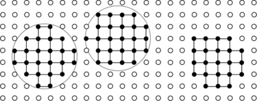
FIGURE 2.34 Gauss digitizations of the same disk at different locations. (In the example on the right, the disk is not shown: this is done to illustrate the difficulty of recognizing digital disks.)
Gauss and Jordan digitization allow us to study methods or algorithms of digital geometry under slightly different assumptions about the relationships between sets S in the Euclidean plane and their digitizations. Evidently, ![]() (and similarly for R3). If S is a nonempty proper subset of R2 or of R3 with a smooth frontier, we have
(and similarly for R3). If S is a nonempty proper subset of R2 or of R3 with a smooth frontier, we have ![]() . Furthermore, the following is true:
. Furthermore, the following is true:
One or both relations ⊆ in the left part of Equation 2.7 can be replaced by =, but both cannot be if S has a smooth frontier. Let S be a finite union of grid squares; then we have J−(S) = G(S) = J+ (S).
2.3.5 Domain digitizations
In this section, we define a framework for a general class of digitization models. To simplify the discussion, we formulate this framework in n dimensions (n ≥ 1), but our main interest is of course in n = 2 and n = 3.
Let the following be the n-cell centered at the origin o = (0,…,0):
Let ![]() ≠ Πσ ⊆ Πcube…., and consider translates Πσ (q) = {q + p : pΠσ} of Πσ centered at grid points q Zn. (Note that Πσ(q) is the Minkowski sum of Πσ and {q}.) In particular, πcube…. (q) is the n-cell cq centered at q.
≠ Πσ ⊆ Πcube…., and consider translates Πσ (q) = {q + p : pΠσ} of Πσ centered at grid points q Zn. (Note that Πσ(q) is the Minkowski sum of Πσ and {q}.) In particular, πcube…. (q) is the n-cell cq centered at q.
We will use the translates Πσ (q) of Πσ as the domains of influence for digitizations that we call ![]() and
and ![]() For any set S ⊆ Rn,
For any set S ⊆ Rn,![]() (q) is the union of all cq such that Πσ (q) intersects S, and
(q) is the union of all cq such that Πσ (q) intersects S, and ![]() (S) is the union of all cq such that Πσ (q) is contained in S. Thus the following is true:
(S) is the union of all cq such that Πσ (q) is contained in S. Thus the following is true:
So ![]() (S) is called the outer σ-digitization of S and
(S) is called the outer σ-digitization of S and ![]() the inner σ-digitization of S. Evidently, for any S ⊆
the inner σ-digitization of S. Evidently, for any S ⊆![]() r
r![]() n, we have
n, we have ![]() (S) ⊆
(S) ⊆ ![]() (S) ⊆
(S) ⊆ ![]() .
.
We now show that Jordan and Gauss digitizations are all σ-digitizations and that grid-intersection digitization can also be regarded as a σ-digitization.
• If πσ = Π…. for n = 2,3, we obtain the inner and outer Jordan digitizations such that, for S ⊆ R2 or S ⊆ R3, we have the following:
• If Πσ = {o}, we have Πσ (q) = {q} so that ![]() (S) =
(S) = ![]() (S) for all S ⊆
(S) for all S ⊆ ![]() Rn. For n = 2 or 3, this set is just the Gauss digitization G(S).
Rn. For n = 2 or 3, this set is just the Gauss digitization G(S).
• If Πσ = {(x1,…,xn):∃i(1 ≤ i ≤ n ∧ xi = 0) ∧ max1≤i≤n |xi|≤½}, ![]() is essentially grid-intersection digitization. (It is a union of cross-shapedneighborhoods of grid cells rather than a union of grid points.) If γ is a planar arc or curve and n = 2, it is not hard to see that R(γ) =
is essentially grid-intersection digitization. (It is a union of cross-shapedneighborhoods of grid cells rather than a union of grid points.) If γ is a planar arc or curve and n = 2, it is not hard to see that R(γ) = ![]() (γ), provided γ does not intersect any grid line midway between two grid points.10
(γ), provided γ does not intersect any grid line midway between two grid points.10
Thus the Jordan digitizations are σ-digitizations in which Πσ is a cube; Gauss digitization is a σ-digitization in which Πσ is a point; and grid-intersection digitization is essentially a σ-digitization in which Πσ is a cross. Other digitization models can be defined by using other simple sets Πσ (e.g.,“ball digitization” by using Πσ = {(x1,…,xn):![]() }, ‘diamond digitization” by using Πσ = {(x1,…,xn): max{|x1|,…,|xn|, 1/(n−1)
}, ‘diamond digitization” by using Πσ = {(x1,…,xn): max{|x1|,…,|xn|, 1/(n−1)![]() These digitizations are illustrated in Figure 2.35. The figure also illustrates a general property that follows directly from the definitions of digσ+ and
These digitizations are illustrated in Figure 2.35. The figure also illustrates a general property that follows directly from the definitions of digσ+ and ![]() and
and ![]() :
:

FIGURE 2.35 Inner and outer diamond and ball digitizations in the plane. The inner digitization is the union of the grid squares centered at black grid points, and the outer digitization (frontier shown as a bold black line) also contains the grid squares centered at shaded grid points. Left: diamond digitization. Right: ball digitization.
2.4 Property Estimation
In Section 2.3.3, we briefly discussed the estimation of arc length from a grid-intersection digitization. In this section, we discuss area and perimeter estimation from a Gauss digitization and introduce the general concept of multigrid convergence of property estimates.
2.4.1 Content estimation
Any simple grid polygon P has a well-defined area and perimeter. The area A(P) is defined by the number of grid squares contained in P multiplied by h−2, which is the area of a single grid square. The perimeter P(P) is defined by the number of grid edges that form the frontier of P multiplied by 1/h, which is the length of a single grid edge. These measurements are invariant with respect to rotations and translations.
A grid polyhedron is simple iff it is topologically equivalent to a closed sphere. (For topologic equivalence, see Chapter 6.) The surface area S (Π) and the volume V (Π) of a simple grid polyhedron Π are defined by the number of 2-cells that form the frontier of Π multiplied by h−2 and the number of 3-cells contained in Π multiplied by h−3, respectively.
The question arises whether these properties of grid polygons or grid polyhedra can serve as estimates of the corresponding properties of real objects that have the polygons or polyhedra as their digitizations. Such estimates can be evaluated using criteria such as absolute error or bias (for a fixed h) or convergence (as h → ∞).
Let S ⊂ rn (n ≥ 1) be a closed bounded set that has measurable content C(S), which is the length L(S) for n = 1, the area A(S) for n = 2, and the volume V(S) for n = 3. We consider a fixed grid constant 1 and magnifications of S by factors h gt; 1. (Our preferred model of a fixed set S and increases in the grid constant will be used in Section 2.4.2.) Let N (S)= C (G(S)) be the number of grid points in S; this is defined by its Gauss digitization in the n-dimensional orthogonal grid.
Suppose Sh depends on only one parameter h gt; 0 (e.g., a disk or a sphere depends on its radius h). Then the following is true as h →∞:
Magnification of S by the factor h with respect to the origin O ∈ Rn transforms S into Sh. (Magnification was defined in Section 2.3.2 only for n = 3, but its generalization to any n ≥ 2 is straightforward.) For n = 2, we have [616, 1023] the upper bound
where P(S) ≥ 1 is the perimeter of S, assuming that S has a rectifiable frontier.11The following general upper bound (for n > 2) was claimed by R. Lipschitz (1832–1903) in [658]:
in a recent letter to him. Let J be a closed rectifiable Jordan curve of length l, enclosing an area a. Then, provided l > 1, the number w of points with integral coordinates inside J satisfies | w – a| l. The proof is elementary and depends on the following result: if a Jordan arc S joins two points on the boundary of the square ![]() , dividing the square into two regions, and if Δ is the region which does not contain the origin, then the area of Δ is less than the length of S. This is proved by simple considerations in each of four possible cases.” The following general upper bound (for n > 2) was claimed by R. Lipschitz (1832–1903) in [658]:
, dividing the square into two regions, and if Δ is the region which does not contain the origin, then the area of Δ is less than the length of S. This is proved by simple considerations in each of four possible cases.” The following general upper bound (for n > 2) was claimed by R. Lipschitz (1832–1903) in [658]:
where Q is the greatest (n − 1)-dimensional content of any of the projections of S into the (n − 1)-dimensional subspaces of Rn defined by xi = 0(i = 1,…,n) and c is a positive constant. Without discussing constraints on the set S, it was pointed out in [248] that this upper bound cannot be correct; in fact, it fails for a long thin cylinder around one of the coordinate axes, where N(S) can be arbitrarily large and C(S) and Q can be arbitrarily small.
Suppose the bounded closed set S ⊂ Rn is such that the following are true: (i) any line parallel to one of the coordinate axes intersects S at a set of points that (if it is not empty) consists of at most t intervals; and (ii) the same is true (with m in place of n) for any of the m-dimensional sets (m = 1,…,n−1) obtained by projecting S into a subspace defined by setting any n – m coordinates to zero. Then we have the following:
Theorem 2.1
(H. Davenport, 1951) If a bounded closed set S satisfies (i) and(ii), then ![]() where Qm is the sum of the m-dimensional volumes of the projections of S on the subspaces obtained by setting any n – m coordinates to zero; t is the maximum number of intervals in (i) for all m = 0,…,n − 1; and Q0 = 1 by convention.
where Qm is the sum of the m-dimensional volumes of the projections of S on the subspaces obtained by setting any n – m coordinates to zero; t is the maximum number of intervals in (i) for all m = 0,…,n − 1; and Q0 = 1 by convention.
Note that t does not change when S is magnified by a factor h (e.g., with respect to the origin).
The n-dimensional content of S ⊂ Rn is the zero-order moment of S (see Chapter 17). Error estimates for content and for digital moments are a general topic in number theory. For information about error estimates for digital moments when n = 2, see Theorems 17.2 and 17.3.
2.4.2 Convergent 2D area estimates
A (real) disk of unit diameter has A(D) = π/4 and P(D) = π. The area of a digitized disk converges toward the area of the real disk:
On the other hand, the perimeter of the digitized disk is always equal to 4, because the total length of the isothetic edges on its frontier remains constant as h increases; thus it trivially converges, but not toward the correct value P(D) = π.
Digital geometry should provide accurate estimates of quantitative properties of digitized sets if the grid resolution is sufficiently large. The study of the accuracy of such estimates is one of the main topics in this book.
Estimation of the area of a planar set by the number of grid points contained in the set has an extensive history in number theory. C.F. Gauss and his colleague P. Dirichlet (1805–1859) at Göttingen University already knew that the number of grid points (i,j)Z2 inside h · S (the magnification of a given planar convex set S by factor h) estimates A(h · S) within an asymptotic order of O(P(h · S)). Note that, because S is convex, P(h · S) is O(h).
Let S be a convex set contained in a unit square so that P(S) ≤ 4 =O(1), and consider increases in the grid resolution h instead of magnifications by an increasing factor h. A(Gh(S)) is estimated by the number of grid points (i/h,j/h) inside S times the scale factor h−2; note that h−2 is the size of a 2-cell in Gh(S). Then we can rewrite the historic result as follows:
Theorem 2.4
Let S be a planar convex 3-smooth set. Then, for grid resolution ![]()
As we have seen, estimates of perimeter require more advanced methods than simply taking the perimeters of isothetic polygons. Such methods will be discussed in Chapter 10.
2.4.3 Multigrid convergence
A general scheme for comparing measurements made on a digital picture subset with the true measurements for the preimage of the subset in Euclidean space has been formalized by J. Serra [969]. (Limit properties with respect to digitizations were also studied in [740] by U. Montanari.)
Let F be a family of sets S in Rn, and let digh (S) denote a digitization of S on a grid of resolution h. Assume that a property Q (e.g., area, perimeter) is defined for all S ∈F. The following definition specifies also a measure of the speed of convergence of a digital quantity toward the true quantity:
Definition 2.10
An estimator EQ is multigrid convergent for F and for digh iff, for any S ∈ F, there is a grid resolution hs > 0 such that the estimated value EQ(digh(S)) is defined for any grid resolution h ≥ hS, and
whereκ is a function defined on the real numbers that takes on only positive real values and converges to zero as h → ∞. The functionκ specifies the speed of convergence.
In Theorems 2.2, 2.3, and 2.4, F is the set of planar convex 3-smooth sets, digh is the Gauss digitization Gh, and Q is the area A. The estimate Ea is obtained by counting the number of grid points scaled by the area of the 2-cells. Theorems 2.2 and 2.4 demonstrate progress in obtaining upper bounds on the convergence speed, and Theorem 2.3 provides a lower bound. The actual convergence speed is between these bounds and is still unknown.
There are two ways to study convergence with respect to increased grid resolution: either consider sets h · S digitized on a grid with unit grid constant, or consider sets S digitized on grids with grid constant 1/h. In both cases, h →∞ corresponds to an increase in grid resolution; we consider either a repeatedly magnified h · S in the grid with unit grid constant or a fixed S in a repeatedly refined grid. The repeatedly refined grid approach is commonly used in numeric mathematics and is also the preferred approach in this book. This is motivated by the assumed scenario in which the set to be analyzed remains physically the same while improvements in hardware (e.g., scanners, computing power) allow refinements in grid resolution. However, in experiments on multigrid convergence, it is often more appropriate to use repeatedly magnified sets digitized into pictures of increasing size.
2.5 Exercises
1. A spider sitting on the surface of a cubic room wants to crawl over all six faces of the cube and return to its starting point as quickly as possible. Does the starting point affect the length of the shortest path?
2. Prove that there is no equilateral triangle that has all three of its vertices in Z2 (see also Exercise 15 in Section 1.3) but that there are equilateral grid triangles in Z3.
3. Use the 12 free 5-ominoes (see Figure 2.20) to cover a 6 × 10 rectangle without overlap. (Hint: All congruence transformations are allowed.)
4. The following figure shows a convex polygon S and its digitization Gh(S). In this example, Gh(S) consists of two rectangles. Give conditions on a bounded convex polygon S and on the grid resolution h gt;0 that imply that Gh(S) consists of exactly one simple isothetic polygon. (For example, this is true if S is an isothetic rectangle.)

5. Construct Gauss digitizations of a square (of constant size) in different orientations using grid resolution 6. Draw a diagram showing the relative deviations of the area and perimeter of the digitized square as a function of its orientation.
6. Consider a polygonal arc with vertices that are grid points and with endpoints that are on the border of Gmn so that the arc cuts Gm,n into two parts. Write a program to determine whether the parts can be moved apart (as in the three cases on the left in the figure above) or not (as in the three cases on the right). (Hint: If so, they can be moved apart by sliding them in the direction of one of the arc segments.)
7. When we use the coding scheme of Figure 2.31, adding 2 modulo 8 to all of the directional codes results in a 90 rotation of the curve. Give an example of a digital curve for which adding 1 modulo 8 to all of the codes results in a digital arc that is not a closed digital curve. (It follows that the addition of 1 modulo 8 does not result in a 45 rotation.)
8. Define a code for the frontier of a free polyomino consisting of the numbers of 2-cells incident with the vertices of the polyomino when the vertices are visited by scanning the frontier of the polyomino in clockwise order. For example, 113131121312 encodes the free 5-omino shown on the right in Figure 2.21 when the scan starts at the upper left vertex. Any cyclic permutation of this code represents the same free polyomino with respect to a different starting vertex. Define the vertex chain code (VCC) of the free polyomino as the smallest integer that can be generated in this way. (In our example, it is 112131211313.) Prove that, for any free polyomino, the sum of the codes in a VCC of length n is 2n − 4.
9. Let n be the length of the VCC (see Exercise 2.8) of a given free m-omino M, and let c be the number of 1-adjacent pairs of 2-cells in M. (For example, c = 4 for the free 5-omino shown on the right in Figure 2.21.) Prove that 2c + n = 4m.
10. Let γ be the straight line y = x +ε. How does the value of ε affect the digitizations J+ (γ), R(γ), andρ(γ)?
11. Show that the 2D cross digitization of any planar convex set is either empty or a polygonally connected set (see Exercise 4 in Section 1.3).
12. How large should h be to achieve the same accuracy of π = 3.14 that Archimedes obtained if the perimeter of the convex hull of Gh(D) is used for the perimeter estimation of D where D is the unit disk? (Hint: The answer can be found by implementing Graham Scan [see Section 1.2.9] using the leftmost and rightmost vertices in all the rows of the grid that intersect D.)
13. Implement Bresenham’s algorithm (see Algorithm 2.3) and measure the length of the digital segment by initializing a variableLest as 0 and adding 1 for every isothetic step and ![]() . for every diagonal step. Calculate the relative deviation between Lest and de (p, q) (the length of the real segment pq) for different slopes of pq. Which slopes produce maximum deviations?
. for every diagonal step. Calculate the relative deviation between Lest and de (p, q) (the length of the real segment pq) for different slopes of pq. Which slopes produce maximum deviations?
14. The circle (x – xc)2 + (y – yc)2 = r2 can be digitized by using the formula y = yc± (r2 – (x – xc)2)1/2, which defines (in general) two y-values for every integer x in [xc – r,xc + r]. Alternatively, each grid line that intersects the circle is perpendicular to a diameter of the circle that divides the grid line into two rays. Usually there exists a grid point on each of these rays that minimizes the residual |(x2 – xc)2 + (y – yc)2 – r2|; these minimum-residual grid points also define a digitization of the circle. Characterize positions of (xc,yc) and values of r for which the minimum is not unique.
15. Prove that the residual |x2 + y2 – r2| is never the same for adjacent grid points on a grid line if r2 is an integer. It follows that the minimum is unique whenever (xc,yc)∈Z2 and r2∈Z.
16. The digital circle produced by the minimum-residual method has a sharp corner iff three of its consecutive grid points form a right angle; this can happen only at octant frontiers. The figure below illustrates a sharp corner when r = 4 and shows that no sharp corner exists when r = 9. Prove that sharp corners occur iff either there exists an integer x > 0 such that r2 = x2 + x + 1 or there exists an integer y >0 such that r2 = 2y2 − y + 1.

17. Let (xc,yc) = (0,0) and r ∈ Z, and suppose (xi,yi) (i ≥ 1) is a grid point on the digital circle generated using the minimum-residual method, where (x1,y1) = (0,r) and xi r. Suppose the (upper) ray at x = xi intersects the circle at (xi,y), where y ∈ R. Let d1,i = ![]() –y2, d2,i = y2 – (
–y2, d2,i = y2 – (![]() − 1)2, and ei = d1,i – d2,i. Prove the following:
− 1)2, and ei = d1,i – d2,i. Prove the following:
Show how these error calculations can be used to generate a digital disk using the given formulas in the second octant and using reflection in the remaining octants.
18. Let S be a measurable set in R2 with a frontier that is a rectifiable simple closed curve. Let A(S) be the area of S and P(S) its perimeter. We recall (see Section 1.2.11) that P2(S)/A(S) ≤ 4π and = 4π iff S is a disk. Let M be a finite set of grid points; define A(M) as the number of grid points in M and P(M) as the number of border grid points in M (i.e., grid points of M that are adjacent to ![]() ). Show that P2(M)/A(M) does not take on its minimum value when M is the set of grid points of a digitized disk.
). Show that P2(M)/A(M) does not take on its minimum value when M is the set of grid points of a digitized disk.
2.6 Commented Bibliography
Both 2D and 3D regular orthogonal grids have a long history (see Figure 2.36). Adjacency grids have been basic models in digital geometry since its beginnings (see [881, 886] for the crisp case and [895] for the fuzzy case). Switch adjacency was defined in [545]. Reference [721] also defines an adjacency relation that is intermediate between 4- and 8-adjacency.
FIGURE 2.36 A figure from Euclid’s ‘Elements,” Book XI, Propositions 31 through 33 about the volumes of parallelepipeds (today we might call them ‘face-adjacent 3-cells”).
For incidence grids (also called the cuberille model) see, for example, [432]. Interestingly, 2D (regular orthogonal grid) incidence was briefly introduced in an exercise in [13].
The theory of polyominoes (see [368, 563]) goes back about 100 years. For a brief review of this theory, see Chapter 12 (by D.A. Klarner) in [371]. See [59, 262] for reconstructions of convex polyominoes from orthogonal projections (which are further discussed in Section 14.7), and see [61] for permutations and generation of polyominoes.
[873] and [976] are reviews of component labeling and region adjacency graph construction for 2D and 3D adjacency grids. The Rosenfeld-Pfaltz algorithm was originally formulated for binary pictures only [921]; it is compared in [674] with two other techniques. Linear-time component labeling algorithms that can handle a variety of image representations are described in [269]; see also [1049]. For component labeling in 3D, see [673, 1053]. The recursive fill algorithm is standard in the picture analysis and computer graphics literature; see, for example, [802]. Component labeling for pictures of very large size can be based on the reuse of labels [506]. For other references about component labeling see [161, 260, 321, 663, 981].
Parallel algorithms for component labeling are discussed in [645, 769, 898]. Connected components can also be determined by identifying borders and computing their chain codes; see, for example, [169, 230, 602, 1034] for early work. (Border tracing is discussed in Section 4.3.4.)
The Gauss digitization model is common in number theory [598]. The Jordan digitization model [484] has been used in connection with volume estimation [732, 960]. Outer Jordan digitization is called super-cover digitization in [209].
Grid-intersection digitization is used in both computer graphics [121, 122] and picture analysis [342, 343, 804, 883]. Bresenham’s algorithm [122] was published in 1965 and is one of the most frequently applied algorithms worldwide. Two versions of grid-intersection digitization are discussed in [951]. For a fast algorithm for grid-intersection digitization of analytically defined curves, see [1032]. The accuracy and time complexity of two line-digitization algorithms are discussed in [1084].
The directional encoding scheme illustrated in Figure 2.31 was proposed by H. Freeman in [342]. Differential chain codes (differences between pairs of successive codes) were proposed in [805]. [859] discusses measures for comparing chain codes.
The upper bound in Equation 2.6 is studied in [1167]. For determining whether a given finite set of grid points is a digital disk or a digital square, see [512] and [765], respectively. For characterizing digitizations of simple shapes such as disks, squares, and triangles, see also [22, 277, 763, 764, 813, 896, 1132].
Digitization schemes based on intersections with domains (e.g., a closed convex set; a square or cube, in Jordan digitization) are studied in [21, 480, 540, 739, 998, 1000]. Domain digitization is also called ‘digitization by dilation and by erosion”[875]. For digitization by dilation, see [416, 417, 419]; here one usually makes the covering assumption, namely that the union of all Πσ (p), for all p∈Z2, covers the Euclidean space. For 2D digitizations based on percentages (ratios of areas within a 2-cell), see [398]. For digitizations of line drawings, see [345, 583]; the special case of convex curves is studied in [1139]. [131] studies digitization schemes, for example, for straight lines and planes from topologic points of view. For Hausdorff digitization, which uses the Hausdorff distance (see Chapter 3), see [875, 876, 1043, 1044]. Digitization is also discussed in [361] and [624] in the context of topology and shape preservation.
Theorem 2.3 is from [412], and Theorem 2.4 from [459]. Definition 2.10 follows [498, 560]. Limit properties of digitization schemes are discussed in [740, 969]. The estimation of radii of digital disks is studied in [1132], of areas of digital disks and rectangles in [878], and of parameters of digital conics in [176]. [556] gives a set of axioms for area measures. For areas and perimeters of digitized objects, see [607].
Exercise 6 is from the 2002 international programming contest of the Association for Computing Machinery (ACM). Exercise 7 is from [1024]. For the vertex chain code and Exercises 8 and 9, see [126]. A chain code for 6-curves (in 3D space) based on a notation for turns is discussed in [127]. Methods of generating digital circles (see Exercises 14 and 16) are discussed in [712]. The result of Exercise 15 is from [606]; see also [178, 276, 813] for digitizations of disks. Exercise 17 is a brief sketch of the basic steps of Bresenham’s digital circle algorithm [123]. The minimum-residual method coincides with grid-intersection digitization for circles that have integer radii and are centered at grid points; see [712]. For the digital isoperimetric inequality (Exercise 18), see [884].
1Half-integers can be avoided in a computer program, for example, by identifying the corners of voxel (i, j, k) with (i + 1, j, k), (i, j + 1, k), (i + 1, j + 1, k), and so on; however, we find it convenient to use half-integer grid vertices in this book.
2pq is the line segment with endpoints p and q, pqr is the triangle with vertices p, q, and r, and so forth.
3In optics, resolution is defined as the minimal distance between two point light sources that allows them to be distinguished by the optic system. In our terminology, resolution is the physical size of a pixel (i.e., the grid constant θ).
4Note that the large squares and thin rectangles are topologically closed sets; however, they represent grid squares and grid edges that are open sets (i.e., the squares do not contain their edges, and the edges do not contain their endpoints). This representation will be convenient when we define topologic equivalence in Chapter 6, because the squares and rectangles used in the representation are all compact (closed and bounded) sets.
5For properties of a set that are invariant under specific types of geometric transformations, see Section 1.2.2 and Chapter 14.
6The FILL algorithm in Algorithm 2.1 uses a depth-first strategy to visit all of the pixels in a component. The books [773] and [805] discuss variants of this strategy, such as recursive and nonrecursive (i.e., ‘filling by connectivity”). The time complexity of this strategy can be improved by stacking horizontal runs of pixels [873]. In some versions of the FILL algorithm, the stack is replaced by a first-in-first-out queue. See Chapter 4 for a generalization and modifications.
7Standard graph traversal algorithms (e.g., depth-first, breadth-first) can also be used to find the labels equivalent to a given label. Graphs are the subject of Chapter 4.
9Precise definitions of curves and arcs will be given in Chapters 6, 7, and 8. For the moment, we say that a simple arc or curve intersects the lines of a 2D grid (or the planes of a 3D grid) a finite number of times.
10In this situation, two grid cells must be added to ![]() , but only one to R(γ). However, this technical difference could be removed by a simple modification of πσ: we require that −1/2 ≤ xi 1/2 (i.e., πσ is a product of n − 1 half-open segments).
, but only one to R(γ). However, this technical difference could be removed by a simple modification of πσ: we require that −1/2 ≤ xi 1/2 (i.e., πσ is a product of n − 1 half-open segments).
11H. Davenport reviews [1023] as follows in Mathematical Reviews, 9:335d: “The author gives a proof of the following theorem, stated and proved by V. Jarník in a recent letter to him. Let J be a closed rectifiable Jordan curve of length l, enclosing an area a. Then, provided l ≥ 1, the number w of points with integral coordinates inside J satisfies | w – a| l. The proof is elementary and depends on the following result: if a Jordan arc S joins two points on the boundary of the square ![]() dividing the square into two regions, and if Δ is the region which does not contain the origin, then the area of Δ is less than the length of S. This is proved by simple considerations in each of four possible cases.”
dividing the square into two regions, and if Δ is the region which does not contain the origin, then the area of Δ is less than the length of S. This is proved by simple considerations in each of four possible cases.”