
Hulls and Diagrams
The convex hull of a set can be regarded as a “domain of influence” of the set. Similarly, the Voronoi diagram of a set of points defines “domains of influence” of the points. This chapter discusses hulls and diagrams in Euclidean space or in a grid, with emphasis on 2D. We discuss definitions of digital convexity and digital Voronoi diagrams and give algorithms based on adjacency grid models. We also discuss “domains of influence” in pictures.
13.1 Hulls
Let S be a class of subsets of a set S. A function H that takes sets in S into sets in S is called a hull operator iff it has the following properties:
H1 and H3 imply that H (H (M)) = H (M) (i.e., H is an idempotent operator). A hull operator is also called a closure operator in algebra. The identity operator I(M) = M and the topologic closure are examples of hull operators. In the following examples, S is Euclidean space Rn.
1) Let S = ![]() (S) be the class of all subsets of S. M ⊆ S is called convex if, for any distinct p, q ∈ M, the straight line segment pq is contained in M. It is easy to see that any intersection of convex subsets of S is convex. The intersection C(M) of all of the convex subsets of S that contain M is called the convex hull of M. It is not hard to show that C is a hull operator.
(S) be the class of all subsets of S. M ⊆ S is called convex if, for any distinct p, q ∈ M, the straight line segment pq is contained in M. It is easy to see that any intersection of convex subsets of S is convex. The intersection C(M) of all of the convex subsets of S that contain M is called the convex hull of M. It is not hard to show that C is a hull operator.
2) Let S be the class of all bounded subsets of S. For any M ∈ S, let De(M) be a disk of smallest radius (defined by metric de) that contains M. Such a disk is not necessarily uniquely defined, but the smallest radius is uniquely defined, because the radius is a continuous function on the compact set defined by the closed convex hull of the set. It is not hard to see that De satisfies H1 and H3 but not H2 (see Figure 13.1). Such an operator is called a pseudohull. Similar remarks apply to the operator R for which R(M) is the rectangle of smallest area that contains M. (Note that R(M) may also not be unique, for example, if M is a disk; to make it unique, we can also require that one of its sides make the smallest possible angle with the positive x-axis. As in the previous argument for the radius, the smallest area is also uniquely defined.) It can be shown that these operators also satisfy the following:

FIGURE 13.1 Left: De({p1, p2, p3}) is not contained in De({p1,…, p4}). Right: R({q1,…, q4}) is not contained in R({q1,…, q6}).
Note that this axiom also implies that H (M) is measurable for M ∈ S. An operator that satisfies H1, H3, and H4 is called a near-hull. H2 implies H4 for any family S of sets S such that H (S) is always measurable.
3) Let S be the class of all finite subsets of S that contain at least two points. For any M ∈ S and any p ∈ M, let ![]() be a disk of smallest radius centered at p that contains another point q of M. Let
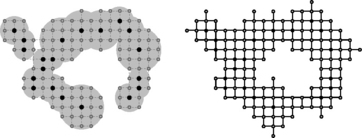
be a disk of smallest radius centered at p that contains another point q of M. Let ![]() . It is not hard to show that Ee is a near-hull. Figure 13.2 (left) shows (in gray) the Ee-hull of a set of grid points (the filled dots). Figure 13.2 (right) shows the E4-hull of the same set of points defined using d4 “disks” (diamonds centered at the points).
. It is not hard to show that Ee is a near-hull. Figure 13.2 (left) shows (in gray) the Ee-hull of a set of grid points (the filled dots). Figure 13.2 (right) shows the E4-hull of the same set of points defined using d4 “disks” (diamonds centered at the points).
H.W.E. Jung [485] analyzed balls Be(M) with smallest radius in Rn (i.e., the generalization of disks of smallest radius to n dimensions [n ≥ 2]). He showed that, if M ⊂ Rn is finite and has diameter d, the radius of Be(M) is upper bounded by the following:
An example for n = 2 is shown in Figure 13.3. A disk of radius d centered at any of the points of M must contain M. Let p,q ∈ M be two points such that de(p, q) = d. Draw two disks of radius d centered at p and q. Because M lies in each disk, it lies in their intersection, which is shaded in the figure. The bold circle contains the shaded region and has radius ![]() . Jung’s theorem shows that this bound can be reduced to
. Jung’s theorem shows that this bound can be reduced to ![]() . Jung’s upper bound is the best possible; there are finite sets M ⊂ R2 for which De(M) has exactly this radius. The radius of De(M) also has the trivial lower bound d/2.
. Jung’s upper bound is the best possible; there are finite sets M ⊂ R2 for which De(M) has exactly this radius. The radius of De(M) also has the trivial lower bound d/2.

13.1.1 Convex hull computation in the Euclidean plane
Let Π be a simple polygon in the Euclidean plane together with its interior, and let ![]() (n ≥ 3) be the vertices of Π. It is not hard to show (see Section 1.2.9) that the convex hull of Π is a polygon and has m ≤ n vertices. In this section, we show how to compute the vertices q1,…, qm of C (Π).
(n ≥ 3) be the vertices of Π. It is not hard to show (see Section 1.2.9) that the convex hull of Π is a polygon and has m ≤ n vertices. In this section, we show how to compute the vertices q1,…, qm of C (Π).
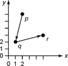
We use the determinant D(p, q, r) (see Equation 8.14,) to classify triples of successive vertices p,q,r of Π as negative if p,q,r is a right turn; zero if p, q, and r are collinear; and positive if p,q,r is a left turn. Figure 13.4 shows an example of a left turn for which D(p,q,r) = 15. In convex hull algorithms, we use the notation D(p, q,r) = L and D(p, q,r) = R for left and right turns.
We use a stack for the vertices of C(Π). At a given step of a convex hull algorithm, the stack contains, for example, q0, q1,…, qt so that its depth is t + 1. The operation PUSH (p) means that t becomes t + 1 and p becomes the last element of the stack. The operation POP means that t becomes t −1 by removal of qt from the stack. p ← p + 1 denotes a move to the next vertex of Π.
We assume that p1 is known to be a vertex of C(Π); for example, we can choose p1 to be the uppermost of the leftmost vertices of Π. Sklansky’s algorithm [999] for calculating C(Π) is shown in Algorithm 13.1. This algorithm has computation time linear in the number of vertices of Π. It is correct provided that the frontier of Π is completely visible from the outside (i.e., through any point q on the frontier of Π there is a ray that intersects Π only at q). Step 4 of Graham’s Scan (see Algorithm 1.1) also assumes that the simple polygon is completely visible from the outside.
Figure 13.5 shows an example of a simple polygon that is not completely visible from the outside. Sklansky’s algorithm fails for this polygon. The algorithm starts at p1 and proceeds correctly up to p5 but cannot deal properly with p6.(A concavity in Π is the closure of a connected component of C(Π)Π. It is not hard to see that a concavity of a polygon is a polygon. An edge of a concavity closes the concavity iff it is not an edge of Π. When the tracing of the frontier of Π goes from p6 to p7, it crosses p2p5, which is an edge that closes a concavity in Π.)
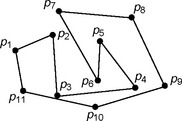
One way to correct the behavior of Sklansky’s algorithm is to continue tracing the frontier (doing nothing to the stack) until p2p5 is crossed again, and then resume with the algorithm until another concavity is found. An algorithm that uses this strategy is shown in Algorithm 13.2. Here we use the Boolean variable flag to indicate whether the vertex tracing is outside a concavity (flag = 0) or inside a concavity (flag = 1). p* denotes the vertex immediately preceding p on Π. This algorithm has linear time complexity.
The situation is more complex if the input is not an ordered sequence of vertices of a simple polygon but rather a set of n points in the plane. In this situation, the worst-case time complexity of any convex hull algorithm is Ω(n log n). In fact, there exist optimal algorithms that have a worst-case complexity of O(n log n); Graham’s Scan (Section 1.2.9) is such an algorithm.
Evidently, the convex hull of a set of n points is a polygon that can have as many as n vertices. It can be shown [847] that the expected number of vertices of the convex hull of a set of n points is ![]() if the n points are independently and uniformly distributed in a bounded convex r-gon; it is O(n1/3) if they are independently and uniformly distributed in a bounded, simply connected set that has a smooth frontier; and it is
if the n points are independently and uniformly distributed in a bounded convex r-gon; it is O(n1/3) if they are independently and uniformly distributed in a bounded, simply connected set that has a smooth frontier; and it is ![]() if their distribution is Gaussian.
if their distribution is Gaussian.
13.1.2 Convex hull computation in the (2D) grid
Knowing that the vertices of a simple polygon have integer coordinates (i.e., that it is a grid polygon) results in no asymptotic time benefit for convex hull computation, but methods of convex hull computation exist that are applicable only to grid polygons. For example, the leftmost (downward) and rightmost (upward) 1s in each row of Figure 13.6 can be used as an input sequence for Sklansky’s algorithm; they form a

FIGURE 13.6 An 8-connected set in which we first identify extreme pixels in each row (pixel p is extreme in both directions) and then apply Sklansky’s convex hull algorithm.
polygon that is completely visible from the outside. Note that this polygon may not be simple (see pixel p).
This algorithm can be applied even if the set of 1s is 8-disconnected. Let xmax, xmin, ymax, and ymin be (estimates of) the greatest and least coordinates of all the 1s. (Exact values of these quantities can be calculated in time linear in the number of 4-border pixels of a region by adding four counters to the border tracing algorithm; see Algorithm 4.3.) We have to scan m = ymax – ymin + 1 rows of pixels each of length up to n = xmax – xmin + 1 to identify the leftmost and rightmost 1s in each row; this takes O(mn) time. We then apply Sklansky’s algorithm to the sequence of leftmost (downward) and rightmost (upward) 1s; this takes O(max{m,n}) time, which is less than O(mn), so the asymptotic upper time bound is O(mn). On the other hand, if we take all of the 1s in the rectangle as unsorted points and use an optimum-time convex hull algorithm (e.g., Graham’s Scan), we obtain an asymptotic upper time bound of O(mnlogmn), because there may be up to mn 1s in the rectangle. This shows that the optimal-time bound for unrestricted input may not be optimal when the input consists only of grid points.
A convex hull that 1 is a grid polygon and that is contained in the grid Gm+1,m+1 can have only a limited number of vertices. Conversely, let e(m) be the maximum number of grid vertices. Let m = s(n) be the minimal side length of a square with vertices that are grid points and that contains a convex grid polygon that has n vertices. It can be shown that the following is true:
Figure 13.7 shows that e(7) = 13, e(8) = 14, and e(9) = 16; s(13)= 7, s(14)= 8, s(15) = 9, and s(16)= 9. These examples also show that, in convex hulls that have maximal number of vertices, the edges tend to be defined by pairs (a, b) of relatively prime integers, where a and b are the increments in the x and y directions. For example, for n = 8, we have the edges (0,1), (1,1), (2,1), (1,0), (2,−1), (1, −2), (0, −1), (−1, −2), (−1, −1), (−1,0), (−2,1), (−1,1), and (−1,2), which constitute a traversal around the convex hull.
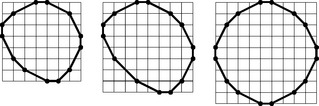
FIGURE 13.7 Three examples of maximal numbers of vertices on a convex hull [1110]. Left: m = 7. Middle: m = 8. Right: m = 9.
In the following discussion, we use Euler’s totient function φ;φ(t) is the number of natural numbers r ≤ t that are relatively prime to t. For example,φ(10) = 4 (r = 1,3,7,9). Note that φ(1) = 1.
We now describe a method of constructing convex hulls that have at most t vertices. Sort all of the pairs (a, b) of relatively prime integers such that a + b ≤ t in decreasing order of the slope of the line segment defined by (a,b) starting at (0,1) and ending at (t − 1,1). There are ![]() pairs (a, b) in this sequence. The polygonal arc defined by this sequence is a quadrant of the convex hull. The example m = 9 in Figure 13.7 illustrates this construction for t = 3. The resulting convex grid polygon has nt = e(mt) = 4.
pairs (a, b) in this sequence. The polygonal arc defined by this sequence is a quadrant of the convex hull. The example m = 9 in Figure 13.7 illustrates this construction for t = 3. The resulting convex grid polygon has nt = e(mt) = 4. ![]() vertices and is contained in a square with vertices that are grid points and that has side length
vertices and is contained in a square with vertices that are grid points and that has side length ![]() . Based on this discussion, we have the following:
. Based on this discussion, we have the following:
Proposition 13.1
There exist strictly monotonically increasing sequences of natural numbers {mt} and {nt}(t = 1,2,3,…) such that the following is true:![]()
In number theory, it is known [991] that, for sufficiently large t, e(mt)/t2 ≈ 12/π2 ≈ 1·2159, s(nt)/t3 ≈ 2/π2 = 0·2026, and s(nt)/e(mt)3/2 ≈ π/12 · 31/2 ≈ 0·1511. Table 13.1 illustrates the speed of convergence of these approximations. Because s and e are monotonically increasing functions (see Exercise 2 in Section 13.4), we can conclude that s(n) ∈ O(n3/2) and e(m) ∈ O(m2/3). More precisely, it can be shown that the following is true:

Table 13.1 shows that e and s intersect between t = 37 and t = 48.
The exponent 2/3 in the estimate of e(m) also occurs in the estimation of the maximal number of grid points on a convex Jordan curve. I.V. Jarnik showed in 1925 [475] that a convex Jordan curve of length l is incident with at most
grid points and that the first term is the best possible upper bound (i.e., there exist curves that achieve this upper bound).
13.1.3 Near-Hull Computation in the Euclidean Plane
In this section, we discuss algorithms for computing the rectangle R(M) with the smallest possible area that contains a finite set of points or a simple polygon M in the Euclidean plane. It can be shown [347] that the following is true:
Proposition 13.2
A side of R(M) is incident with an edge of C(M).
On the basis of this, we can compute R(M) as follows. Let v1 be the first vertex of C(M). Examine the vertices in sequence until the first vertex v2 (not on the first edge) is found such that a line l through v2 parallel to the first edge does not intersect the interior of C(M); see Figure 13.8 (left). Choose vertices v3 between v1 and v2 and v4 between v2 and v1 that define a circumscribing rectangle of M. After this initialization step, move v1 to successive vertices of C(M) and move pointers v2, v3, and v4 (if necessary) so that the four vertices continue to define a circumscribing rectangle. Figure 13.8 (right) illustrates a move of v1. Compare the areas of the resulting rectangles, and choose the smallest one.
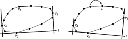
FIGURE 13.8 Vertex v1 moves to the next position and triggers a move of pointer v2; v3 and v4 need not move.
Let n be the number of vertices of C(M). The initialization step takes O(n) computation time; each of the vertices v1,…,v4 moves into at most n positions, and each move takes constant time. Hence the algorithm is linear in the number of vertices on the convex hull (if the initial calculation of C(M) is not taken into account).
Let S be the class of subsets of E2 with frontiers that are Jordan curves so that they are homeomorphic to the unit disk. It can be shown that any M ∈ S has a circumscribing square (i.e., a square with all four edges intersecting M in at least one point). Let Q(M) be the circumscribing square that has smallest area; we can make Q(M) unique by minimizing the angle that one of its sides makes with the positive x-axis. As was the case in Section 13.1, Q(M) defines a near-hull.
Proposition 13.3
Any plane Jordan curve γ has a circumscribing square (i.e., a square that contains γ, with all four sides having a nonempty intersection with γ).
Proof Let l be a line that does not intersect γ and l′ a line parallel to l (e.g., with slope θ) such that γ is in the stripe between l and l′. Move both lines toward γ by parallel translation until they intersect γ for the first time. The resulting lines are lines of support of γ. Similarly, construct two other lines of support that are orthogonal to l. These four lines of support define a circumscribing rectangle of γ. Let the side lengths of this rectangle be a(l) and b(l). If we perform this construction for lines l with slopes between θ and θ + π/2, we obtain circumscribing rectangles with side lengths that change from (a(l),b(l)) to (b(l),a(l)) so that, during the rotation, a(l) – b(l) changes sign. Evidently, a(l) – b(l) is a continuous function of θ.,1 Hence a(l) – b(l) must be zero for some slope between θ and θ + Π/2 so that the circumscribing rectangle for this slope is a square.

1]Let f : R → R be continuous on [a, b] (a < b); let x1, x2 ∈ [a, b] be such that f (x1) > 0 and f (x2) < 0. Then f (x0) = 0 for some x0 ∈ [a,b].
13.2 2D Digital Convexity
Digitally convex sets were defined in Section 2.3.4 with respect to a digitization model. This section assumes the 2D grid point model (i.e., digitizations are subsets of Z2). A digitization by dilation is an outer σ-digitization using domains of influence Πσ (q), where Πσ contains the origin. For example, Gauss, outer Jordan, and grid-intersection digitization are digitizations by dilation. For any digitization by dilation, a finite S ⊂ Z2 is digitally convex iff S is the digitization of its Euclidean convex hull C(S).
The Gauss digitization G(S) of a convex set S ⊆ R2 may not be 8-connected (see Exercise 1 in Section 2.5), but its cross digitization (defined in Section 2.3.5 by generalizing grid intersection digitization to arbitrary planar sets) must be simply 8-connected (see Exercise 4 in Section 2.5). In this section, we use cross digitization in the 8-adjacency grid. A setø ≠ S ⊆ Z2 will be called digitally convex (with respect to cross digitization) iff there exists a convex set M ⊆ R2 such that S = digcross(M).
13.2.1 Digital Convex Hulls
Evidently, any digital straight line (DSL) or straight line segment (DSS) is digitally convex. Moreover, a finite irreducible 8-arc is digitally convex iff it is an (8-)DSS.
Theorem 13.2
A finite set M ⊆ Z2 is digitally convex iff any one of the following is true:
1. M satisfies the chord property.
2. For all p,q ∈ M, at least one DSS that has p and q as endpixels is contained in M.
3. For all p,q,r ∈ M, all of the grid points in the (closed) triangle pqr are in M.
4. Any grid point on the (real) line segment between two grid points of M is also in M.
5. Let [M] be the union of the grid cells that have centers in M. For any two grid points p and q in M, let Mpq be the region surrounded by the frontier of [M] and the real line segment pq; then any grid point in Mpq is in M.
There exist infinite sets M ⊆ Z2 that satisfy the chord property but that are not digitally convex. For example, let H be a halfplane defined by a straight line γ with irrational slope, and let M be the cross digitization of M. If p ∈ ![]() is 4-adjacent to two 4-border pixels of M, M ∪{p} still satisfies the chord property.
is 4-adjacent to two 4-border pixels of M, M ∪{p} still satisfies the chord property.
The Euclidean convex hull C(M) of any M ⊆ Z2 is a convex polygon with vertices that are all 4-border pixels of M. If M is simply 8-connected, 4-border tracing visits all of the 4-border pixels of M in sequence; see the border tracing algorithm in Section 4.3.4. The vertices of C(M) partition this sequence into finite or (at most two) infinite subsequences that start and end at successive vertices of C(M). These subsequences will be called border segments of M.
13.2.2 Row and Column Convexity
S ⊆ Z2 is called row-convex (column-convex) iff each row (column) of the grid contains at most one run of pixels of S. Let M ⊆ E2 be convex, and let G(M) be nonempty and 4-connected. It is not hard to see that G(M) is row- and column-convex. It can be shown [530] that the number b(n) of row-convex (or column-convex) n-ominoes satisfies the following:
(See Equation 2.4 for the number of all n-ominoes.) It can further be shown [69] that the number c(n) of row-column-convex n-ominoes satisfies the following:
A staircase is a 4-arc that has x- and y-coordinates that are monotonically nonincreasing or nondecreasing. The 8-border of a row-column-convex 4-connected set can be partitioned into at most four staircases; see Figure 13.9 for an example. We see from Figure 13.9 (left) that such a set is not necessarily digitally convex.

13.2.3 Fuzzy Digital Convexity
Let the values of the pixels in a picture P be in the range [0,1] so that P defines a fuzzy subset μ of the grid (see Section 1.2.10). P is called μ-convex iff, for all pixels p, q, there exists a DSS with endpixels p and q such that μ(t) ≥ min(μ(p),μ(q)) for all pixels on the DSS.
P is called μ-(8-)connected (see Section 13.3.3) iff, for all pixels p, q, there exists an (8-)path ρ from p to q such that μ(t) ≥ min(μ(p),μ(q)) for all pixels on ρ. Thus μ-convexity can be regarded as a special case of μ-connectedness in which ρ is required to be a DSS.
In Proposition 13.11, we will see that P is μ-connected iff all of its level sets are connected. Similarly, by Theorem 13.2, we have the following:
13.3 Diagrams
Diagrams are defined in metric spaces for countable sets S of “simple” geometric objects such as points, line segments, polygons, polyhedra, and so on. One type of diagram divides the metric space into cells such that each element of S is contained in exactly one cell. Another type connects some pairs of elements of S by line segments.
Let S = {p1,…, pn} be a set of points in the Euclidean plane E2. The Voronoi cell2 of pi ∈ S (i = 1,…, n) is the closure of its zone of influence, which is the set of all points in E2 that are closer (with respect to metric de)to pi than to any other point of S:
Euclidean distance was used in this definition [1101], but Voronoi cells can be defined in any metric space. (The closure of the zone of influence of pi is not necessarily identical to Ve (pi) if de is replaced by another metric on R2, such as a chamfer metric.)
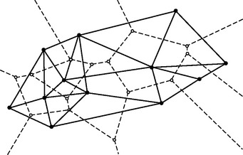
The Voronoi diagram is called the skeleton by influence zones (SKIZ) in mathematic morphology. pi and pk are called Voronoi neighbors iff Ve(pi) and Ve(pk) share an edge (i.e., have more than a single point in common). Distinct Voronoi neighbors are called Voronoi adjacent. The dual Voronoi diagram is obtained by joining the pairs of Voronoi adjacent points with straight line segments. It can be shown that the bounded faces in a dual Voronoi diagram are all triangles iff S is circle-free: whenever more than three points of S lie on a circle, another point of S lies inside of the circle. (Figure 13.10 shows two examples of sets that are not circle-free.) If S is circle-free, its dual Voronoi diagram is called its Delaunay triangulation [259]3; Figure 13.11 shows an example. A dual Voronoi diagram that has edges added to complete a triangulation if S is not circle-free is called a Delaunay diagram.

Voronoi and Delaunay diagrams are well-known examples of diagrams in E2. The Voronoi diagram has a straightforward generalization to En. The set S can be a family of pairwise disjoint simply connected bounded sets rather than a set of points.
Let S be a finite set of points in En. A nearest neighbor diagram of S is defined by the set of (undirected) line segments pq such that p is a nearest neighbor of q in S or vice versa. (In such a diagram, each p ∈ S is joined by a line segment to only one of its nearest neighbors.) A minimum spanning tree diagram is a tree with nodes that are the points of S and with edges that have minimum total length. Note that these diagrams are not necessarily unique; the same is true for Delaunay diagrams of non-circle-free sets.
13.3.1 Diagram Computation in the Euclidean Plane
Let S = {p1…, pn} be a set of points in the Euclidean plane. The Voronoi cells of the points of S are convex. The Voronoi cell Ve(p) is bounded iff p is in the interior of the convex hull C(S). The frontier of an unbounded Voronoi cell consists of at most two straight lines or rays and finitely many straight line segments. A bounded Voronoi cell is a simple polygon. The line segments, rays, or lines on the frontier of a Voronoi cell are contained in the perpendicular bisectors of pairs of points p, q ∈ S; see Figure 13.12.

FIGURE 13.12 The Voronoi diagram is composed of (segments or rays of) perpendicular bisectors. Five “construction steps” for one of the cells are shown; the final Voronoi diagram is at the lower right.
The construction of Voronoi diagrams and Delaunay triangulations are dual processes; either diagram can be derived from the other. We will describe a simple Delaunay diagram construction algorithm that has asymptotic time complexity O(n2) and a small asymptotic constant; it supports time-efficient constructions for (about) n ≤ 1000. For larger sets of points, it is preferable to use optimized algorithms that run in O(n log n) time. The worst-case time complexity of Delaunay diagram construction has lower bound Ω(n log n). If the set of points is not circle-free, the algorithm chooses one of the possible diagrams.
According to Proposition 13.8, a Delaunay diagram is a subdiagram of a nearest neighbor diagram. Given a finite set S of points, we pick a point p in S and search in S for one of the nearest neighbors q of p. We start the construction with pq, which is an edge of one of the Delaunay triangles.
In Figure 13.13, we have the following, where A is the area of triangle pqr:
The points of S are all collinear, for example, on line l, iff A = 0 for all r ∈ S/{p, q}; in this case, the Delaunay diagram connects the points along l in sorted order. From now on, we assume that the points of S are not all collinear.

Points p, q, and r of S form a Delaunay triangle if4 the following is maximal for r among all points of S/{p, q}:
Because c is constant for a given p and q, we need only maximize (a2 + b2 – c2)/A. We recall that ![]() where D is the determinant; see Equation 8.14. This gives us the following test for identifying a third point of a Delaunay triangle:
where D is the determinant; see Equation 8.14. This gives us the following test for identifying a third point of a Delaunay triangle:
Let r ∈ S/{p,q} be the first point for which D(p, q, r) ≠ 0. If D(p, q, r) > 0, we identify third points (throughout the procedure) by maximizing as follows:
If D(p, q, r) < 0, we identify third points by minimizing K(p, q, r).
The sign of D(p, q,r) also tells us whether the ordered triple (p, q, r) describes a left turn or a right turn. The oriented straight line segment from p to q defines two halfplanes; r is in the left (right) halfplane iff (p,q,r) is a left turn (right turn). pq can also be incident with a second Delaunay triangle that has a third point r’ that is in the right (left) halfplane. This is why we put oriented line segments (vectors)
ALGORITHM 13.3 Delaunay diagram algorithm.
1. Choose p ∈ S, and find a q ∈ S that is a nearest neighbor of p. Choose a point t ∈ S/{p, q}; depending on the sign of D(p, q, t), we use maximization or minimization in this run of the algorithm (see text).
2. Find a third point r ∈ S/{p,q} that maximizes (minimizes) K(p, q, r). Put the vectors ![]() ,
, ![]() , and
, and ![]() on a list.
on a list.
3. As long as the list is not empty, go to Step 4; otherwise, stop.
4. Take ![]() off of the list. Set flag := 0, set pointer ThirdPoint := VOID, and set K := −∞ (for maximization) or ∞ (for minimization).
off of the list. Set flag := 0, set pointer ThirdPoint := VOID, and set K := −∞ (for maximization) or ∞ (for minimization).
5. For all r ∈ S/{p, q} (go to Step 6 when finished):
a) If K ≤ K(p, q, r) for maximization or K ≥ K(p, q, r) for minimization, go to Step 5.c.
6. If flag = 0, go to Step 3. Otherwise, let r := ThirdPoint.
//A new Delaunay triangle (p,q,r) has been detected; take appropriate action.//
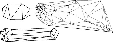
rather than line segments on the list in the algorithm; if we arrive at the same vector a second time, we delete it from the list. The algorithm is given in Algorithm 13.3, and Figure 13.14 shows three examples of Delaunay triangulations.
13.3.2 Diagram Computation in the Digital Plane
If S contains only grid points, only integer arithmetic is needed for Algorithm 13.3 Let G(p,q,r) = a2 + b2 – c2. When we use maximization, the test K(p,q,r1) < K(p,q,r2)? can be replaced with G(p,q,r1) · D(p,q,r2) < G(p,q,r2) · D(p,q,r1)? at the cost of using two variables G and D instead of K.
Sets of grid points are often not circle-free; Figure 13.15 (left) shows an example. However, the Delaunay diagram algorithm (Algorithm 13.3) always produces a triangulation if the points in S are not all collinear. By keeping track of points with equal (maximal or minimal) values of K in Steps 5.a and 5.b, we can also detect points that are incident with more than three Voronoi cells.
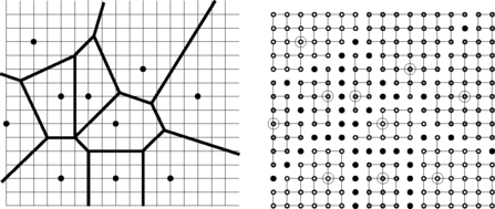
FIGURE 13.15 Left: Voronoi diagram for a set of grid points. The result of the Delaunay diagram algorithm depends on the order in which the points of S are visited, because S is not circle-free (see the Voronoi point that is incident with four Voronoi cells). Right: digital representation of the diagram; grid points on the frontiers of Voronoi cells are black.
In the grid, we are typically interested only in assigning grid points to Voronoi cells or Delaunay triangles. The Euclidean metric was used in Equation 13.4; the resulting Voronoi diagram is called the de-Voronoi diagram; see Figure 13.15, (right). If we use a grid metric dα instead of de in Equation 13.4, we obtain a dα-Voronoi diagram. Figure 13.16 shows d4- and d8-Voronoi diagrams for the set of points used in Figure 13.15.

dα -Voronoi diagrams can be constructed as follows. Initially, we give each point of S a different Voronoi cell label. In each run of the algorithm, we label all of the grid points q that have not yet been labeled but that are α-adjacent to already labeled grid points. If q is α-adjacent only to points that have the same label, give q that label; if q is adjacent to points that have different labels, q is a Voronoi diagram point. Continue this process for as long as unlabeled grid points remain.
For a chamfer metric, the Voronoi diagram can be computed using the Rosenfeld-Pfaltz two-pass distance transform algorithm.
13.3.3 Diagrams in Pictures
Let A be an adjacency relation on a grid Gm,n. An A-path is a sequence of pixels ρ = (p0,…, ph) such that pi is A-adjacent to pi−1 (0 < i ≤ h). Let {S1,…, Sh} be a set of disjoint subsets of Gm,n. A-paths can be used to define “domains of influence” D(Si) of the Sis in various ways. For example, we can say that p belongs to D(Si) iff the length of a shortest path from p to Si is less than the length of a shortest A-path from p to any other Sj (i.e., if p’s “A-distance” to Si is less than its A-distance to any other Sj). If we use this definition, D(Si) is the Voronoi cell of Si with respect to A-distance. (We will usually drop the A in what follows.)
If P is a picture defined on Gm,n, we can restrict the class of allowable paths or assign weights to paths using the values of the pixels on the paths. For example:
a) We can define the value-weighted length of a path ρ as the sum of the values of the pixels of ρ. The value-weighted Voronoi cell of Si then consists of pixels that have a value-weighted distance to Si (see Section 3.4) that is less than their value-weighted distance to any other Sj.
b) We can call ρ allowable iff its pixels all have values greater (or less) than some threshold t. This leads to a Voronoi cell concept based on intrinsic A-distance in the set of pixels that have values that are greater (or less) than t.
c) We can define the slope-weighted length of ρ as the sum of the differences (or absolute differences) of the values of successive pairs of pixels of ρ. (We can think of “steep” paths as taking longer to “climb.”)
d) We can call ρ allowable if its pixel differences all have values greater (or less) than some threshold t. Of particular interest are monotonic paths in which the differences are all nonnegative or all nonpositive.
In the remainder of this section, we will consider only domains of influence defined by monotonic paths, and we will assume that A = A4 or A8.
A maximal (4- or 8-) connected set Π of pixels that has values in P that are constant will be called a plateau5; the constant value will be denoted by P(Π). Evidently, every pixel p belongs to exactly one plateau, which we denote with Π(p).
Two plateaus Π and Π′ are called (4- or 8-) adjacent if some pixel of Π is adjacent to some pixel of Π′. Evidently, if Π and Π′ are adjacent, we must have P(Π) ≠ P(Π′). Π is called a top (bottom) if its value is higher (lower) than that of any plateau adjacent to it. A top is also called a peak or summit and a bottom is also called a pit or sink.
A path ρ =(p0,…, pn) is called nondescending if P (pi) ≥ P (pi−1) and nonascending if P(pi) ≤ P(pi−1) for all 1 ≤ i ≤ n.
We now prove the converse: if P is μ-connected, it must have a unique top. Suppose P had two tops Π and Π′. Let Π0,…,Πn be a sequence of plateaus such that Π0 = Π, Πn = Π′, and Πi is adjacent to Πi−1 (1 ≤ i ≤ n). Choose such a sequence for which min(μ(Πi)) = v is as large as possible and the value v is taken on as few times as possible. Let P (Πj) = v; then, evidently, 0 < j < n and μ(Πj−1),μ(Πj+1) are greater than v. Let Πj−1 and Πj+1 be in μω where ω < v. Because Π is μ-connected,μω must be connected, according to Proposition 13.11. Hence the sequence of Πs can be diverted around Πj through plateaus higher than v; the diverted sequence either has a minimum value higher than v or takes on the value v fewer times, which is a contradiction. We have thus proved the following:
Thus the μ- connected sets of P can be regarded as “domains of influence” of the tops of P.
We now return to the viewpoint from which we regard the pixel values as representing surface heights, and we no longer assume that they are in the range [0,1]. We say that p is directly upstream from q and q directly downstream from p iff P(p) > P(q) and Π(p) is adjacent to Π(q). Evidently, if Π(p) is a top, no q can be directly upstream from p, and, if Π(p) is a bottom, no q can be directly downstream from p. We say that p is upstream from q and q is downstream from p if there exists a sequence of pixels (p0,p1,…, pn) such that p = p0, q = pn, and pi is directly upstream from pi+1(0 ≤ i < n). We can also apply the terms (directly) upstream and downstream to the plateaus themselves.6
Evidently, no pixel can be upstream from a top or downstream from a bottom. On the other hand, according to Proposition 13.9, every pixel either belongs to a top or is downstream from a top, and every pixel either belongs to a bottom or is upstream from a bottom. Note that a pixel may be downstream from more than one top or upstream from more than one bottom. If P is downstream from only one top Π, we say that it belongs to the runoff of Π; if it is upstream from only one bottom Π, we say that it belongs to the watershed (sometimes called the catchment basin) of Π. Let G be the directed graph with nodes that are the plateaus of P and in which (Π, Π′) is a directed edge of G iff Π′ is directly downstream from Π. If Π* is a bottom, p is in the watershed of Π* iff the plateau containing p is connected to Π* in G.
The watersheds of a picture can be identified by assigning a label to each bottom and propagating that label to all of the plateaus that are upstream from that bottom. A pixel p is in the watershed of a bottom Π* if Π(ρ) receives only the label of Π*. A simple picture with pixel values 0,…,4 and the watershed of one of its bottoms (the singleton 0 in the last row) are shown in Figure 13.17. The runoffs of a picture can be identified analogously by assigning labels to the tops.

FIGURE 13.17 A watershed: Left, middle: a picture with pixel values 0, …, 4. Right: the watershed of the 0 in the last row.
In our discussion of runoffs and watersheds, we have ignored the rate at which the surface elevation changes. If q is adjacent to ρ and P(q) < P(p), the rate at which water flows from p to q depends on how much smaller P(q) is than P(p). If p is in the watershed of a bottom Π, there are paths of steepest descent from p to Π. If the edges of G are weighted by their slopes and Π is in the watershed of Π*, we can find strongest paths from Π to Π* (i.e., paths along which the rate of flow of water from Π to Π* is maximal).
A plateau (or pixel) that is upstream from more than one bottom is said to belong to a divide of a surface, because the water that flows from such a plateau is “divided”: it does not all flow to the same bottom. Pixels that lie on the ridges of a surface are usually divide pixels, because the water that flows down the two sides of the ridge usually reaches two or more bottoms. Similarly, pixels that lie in ravines are usually downstream from more than one top, because the water flowing into a ravine from its two sides usually comes from two or more tops. A divide pixel (or plateau) that is directly upstream from pixels (or plateaus) that belong to two different watersheds belongs to the divide line (sometimes called a watershed line) between the two watersheds. If water flowed upward from the bottoms, water from different bottoms would meet at divide lines. Thus there is an analogy between a divide line and a medial axis (see Section 3.4.4) at which the grassfire from the boundary of a set meets itself; however, note that a “divide line” can be very thick, because its pixels can belong to arbitrarily large plateaus. Divide lines that are (usually) not more than two pixels thick can be obtained by using a “viscous” water flow that has a rate that depends on both distance and elevation difference.
13.4 Exercises
1. A shape is a simply connected measurable compact set in the Euclidean plane. For any M ⊆ E2, let S (M) be the smallest shape that is similar to a given shape and that contains M. Which of the properties H1 through H4 are satisfied by the operator S?
2. Let S be the class of all compact subsets of the plane, let M ⊆ S, and let I(M) be the isothetic rectangle of smallest area that contains M. Prove that I is a hull operator.
3. Give algorithms for constructing the smallest circumscribing square or disk of a finite set of points of Z2. (Hint: It is simpler to construct an approximate solution.)
4. Let M ⊂ R2 be finite, let d be its diameter, and let its smallest circumscribing rectangle R(M) have sides of lengths a and b. Find lower and upper bounds for a and b in terms of d.
5. Give examples that show that properties H1, H2, and H3 are independent (e.g., a class S and a mapping H that satisfy H1 but not H2 and not H3).
6. Let Π0 be a simple polygon. We recall (see Section 13.1.1) that a (first order) concavity in Π0 is the closure of a connected component of C(Π0)/Π0. Evidently, Π0 is convex iff it has no first-order concavities. Define a kth-order concavity (k = 2,3,…)in Π0 as a concavity in a (k − 1)st-order concavity in Π0. Prove the following:
a) For any k, kth-order concavities in Π0 are simple polygons with vertices that are vertices of Π0.
b) If k is odd, kth-order concavities in Π are subsets of C(Π0)/Π0; if k is even, kth-order concavities in Π0 are subsets of Π0.
c) If Π0 has n vertices, it cannot have kth-order concavities for k > n. Can you give a better bound on k?
7. Design an algorithm for constructing the convex hull of a finite set S of points in the Euclidean plane using the following strategy. Identify in S the up to eight points that are extreme in the x-, y-, (x + y)-, and (x – y)-directions. Points of S in the interior of the octagon defined by these eight points cannot be on the frontier of the convex hull. The remaining points of S – in addition to the eight points – must lie in eight triangles outside of the octagon. Construct the frontier of the convex hull using only these remaining points.
8. Let e(m) and s(n) be the functions defined in Section 13.1.2. Prove that e(m) ≤ 2m + 2 for ![]() for n ≥ 3; and s and e are monotonically increasing functions.
for n ≥ 3; and s and e are monotonically increasing functions.
9. Show that an 8-disconnected set M can have more than one digitally convex completion.
10. Let dig be a digitization function that maps Euclidean line segments pq ⊂ R2 (p,q ∈ Z2) into 8-regions dig(p, q) ⊂ Z2 such that p, q ∈ dig(p, q). dig is called close iff, for all r ∈dig(p,q), there is a point v ∈ pq such that d8(r,v) < 1, and, for all v ∈ pq, there is a grid point r ∈dig(p, q) such that d8(r,v) < 1. dig is called convex iff, for all r, s ∈dig(p, q), we have dig(r, s) ⊆dig(p, q) for all p,q ∈ Z2. Show that closeness and convexity are mutually exclusive properties of dig.
11. Let M be a finite set of points in R2. If a convex hull edge pq does not intersect “its” Voronoi diagram edge V(p) ∩ V(q), replace pq with two new edges, one of which joins p at the point where the “old” edge pq crosses the frontier of V(p). Continue this process until there is no further change. This process “shrinks” the original convex hull C(M) into a polygon G(M); see Figure 13.18 (left).
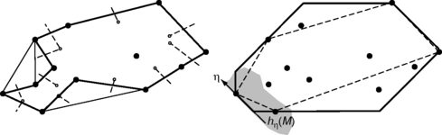
FIGURE 13.18 Left: the bold polygonal line is the frontier of the Gabriel pseudohull; see Figure 13.11 for the Voronoi and Delaunay diagrams. Right: the 8-hull (bold) and 8-approximation (dashed).
(i) Show that G is a pseudohull; it is called the Gabriel pseudohull of M.
(ii) Give an algorithm for calculating the Gabriel pseudohull.
12. Let M ⊂ R2 be finite. The frontier of the 8-approximation of M is defined by the cyclic sequence of points p =(x,y) ∈ M that maximize x, x + y, y, –x + y, –x, –x –y, –y, and x – y, in that order; see Figure 13.18 (right). The 8-hull is defined by intersecting the eight halfplanes defined by tangent lines in directionsη = i2π/8(i = 0,…, 7) that contain M.
(i) Which of the properties H1 through H4 are satisfied by the 8-approximation and the 8-hull?
(ii) Implement the 8-approximation and the 8-hull, generate h points in a square, and compare the mean difference between the areas of their 8-approximation, their 8-hull, and their convex hull (e.g., calculated on the basis of Graham’s algorithm) for h = 100,…, 1000.
13. Let η ∈ [0,2π) be a direction, let p ∈ Z2, and let γη(p) be the oriented straight line through p =(x0, y0) in direction η +π/2 if η ≠ 0 and η ≠ π:![]()
Let it otherwise be as follows:
Let M ⊂ Z2 be finite. p ∈ M is an extreme point of M in direction η (notation: p ∈ Xη (M)) iff M is contained in the closed halfplane hn (M) to the right of γη (p). Let dir(n) =(i2π/n: i = 0,…, n−1} be a set of n directions, and let the following be true:

Hn(M) is the n-hull of M (see Exercise 12 for n = 8), and An(M) is the n-approximation of M.
(i) Extend the experiments of Exercise 12 by comparing the area of the n-hull and n-approximation with the area of the convex hull for n = 4,…, 64.
(ii) Let f (n) be the largest integer m such that, for all finite sets M ⊂ Z2 such that max ![]() , the n-approximation An (M) is always equal to the convex hull C(M). For example, f(1) = 0, f(2)=f(3) = 1, and f(4) = 2. Give lower and upper bounds on f(n) when n is a multiple of 4.
, the n-approximation An (M) is always equal to the convex hull C(M). For example, f(1) = 0, f(2)=f(3) = 1, and f(4) = 2. Give lower and upper bounds on f(n) when n is a multiple of 4.
14. Show that a set S ⊆ Z2 is digitally convex iff there is a supporting (real) line through every point of its 4-border. (Note: Supporting lines of a planar set have the set on one side of them.)
13.5 Commented Bibliography
For a discussion of hulls, pseudohulls, and near-hulls, see [535], which also discusses the Gabriel pseudohull [1062] (see Exercise 10) and the 8-hull [537] (see Exercise 11). The case n = 2 of Jung’s upper bound for the radius of the smallest disk that contains a finite set M ⊂ R2 is also proved in [830]. Relative convex hulls (see Section 1.2.9) define hulls of “inner sets” with respect to a fixed “outer set.” In the context of this chapter, relative convex hulls have applications to analyzing convexity in the grid cell model; see [508]. “Approximate convexity” based on concepts of geometric probability and shape analysis is proposed in [420]. [973] discusses digital “star-shapedness.”
Sklansky’s algorithm was published in [999]. The correct convex hull algorithm for simple polygons (Algorithm 13.1) appeared in [539], thereby correcting an erroneous algorithm in [451]. See the literature about computational geometry (e.g., the textbooks [97, 823] or Chapter 19 [by R. Seidel] in [371]) for other 2D and 3D convex hull algorithms (for simple polygons, finite sets of points, simple polyhedra, and so on). The algorithm sketched in Exercise 6 has linear expected time assuming a uniform distribution of the points in a rectangle [265]. [302] gives expected values of the areas and diameters of the convex hulls of sets of n points.
See [451] for convex hull computation for sets of grid points and [180, 865] for the computation of digital convex hulls. The discussion of maximal numbers of vertices of convex grid polygons in Section 13.1.2 and Exercise 7 follows [1110], which also contains empiric formulas for estimating the functions e and s. See also [465] for asymptotic estimates of e and s. Theorem 13.1 is from [5].
[449] contains a review of digital convexity (see Section 13.2). See [1165] for number-theoretic studies of digital convex polygons. The results in this section are from [348, 451, 510, 515, 516, 854, 911, 952, 998, 999]. See [508, 518] for convexity in the grid cell model. [473] and [1157] discuss fuzzy convexity, and [906] discusses convexity on graphs.
[902] discusses measures of concavity. For more about convex digital regions of specific shapes, see [333,765] (squares) and [276,328,512,606] (disks). See [905] about fuzzy orthoconvexity and rectangles and [906] about fuzzy triangles.
The Delaunay diagram algorithm in Algorithm 13.3 (including the “integer arithmetic only” optimization for sets of grid points) was published in [453]. For a review of Voronoi and Delaunay diagram algorithms (Dirichlet cell algorithms in the general case) and related geometric properties, see Chapter 20 (by S. Fortune) in [371]. For performance analysis of Voronoi tessellation algorithms, see [819]. For Proposition 13.8, see [1062].
An algorithm for Euclidean Dirichlet labeling on Zn (n ≥ 2), assuming a finite set of grid points as input, is given in [373]. The algorithm is based on space-filling curves in Zn; it generalizes examples given in Section 1.1.3 for Z2.
[588] applies dual Voronoi diagrams to the recognition of circular arcs. [119] approximates the skeleton of a set S ⊂ R2 from the Voronoi diagram of points sampled along the frontier of S. [217] studies topologic connectedness in the plane defined by Voronoi cells. For other references regarding Voronoi diagrams, see [8, 38, 310, 385].
For fuzzy connectedness in 2D pictures, see [891, 897]. For classic references about monotonicity-based segmentation of surfaces, see [167, 710]. For watershed segmentation, see [83, 87, 727, 735, 824, 1098]. For Exercise 2 (smallest circumscribing disk), see [1120]. Exercise 9 is from [683], and Exercise 12 follows [537].
2]This is named after the Ukrainian mathematician G.F. Voronoi (1868−1908). An n-dimensional generalization was studied by the German mathematician J.P. G.L. Dirichlet (1805−1859) [273]. The U.S. officer A.H. Thiessen also used such polygonal cells in the discussion of meteorologic data; see, for example, [1050]. Voronoi cells are therefore also called Thiessen polygons and are the 2D case of Dirichlet polyhedra or Dirichlet cells.
3]This is named after the Russian mathematician B.N. Delaunay (also called Delone; 1890−1980).
4]Not “iff,” the line containing p and q defines two halfplanes, and there can be a Delaunay triangle in each of the halfplanes. The maximization can be performed for each halfplane.
5]This terminology is suggested by regarding the picture as defining an isothetic surface in which the value of a pixel defines the height of the surface above the pixel. Plateaus are (4- or 8-) components of P-equivalence classes.
6]This terminology too is motivated by regarding P(p) as the height of a surface above p. If we pour water on the surface at the point above p, it will flow to the point above q iff either q ∈ Π(ρ) or q is downstream from p.