
2D Straightness
This chapter discusses digital straightness in the grid point and grid cell models. We consider its relationships with other disciplines such as number theory and the theory of words as well as its role in picture analysis. We also discuss algorithms for recognizing digital straight line segments (DSSs) and partitioning digital arcs into such segments.
9.1 Basics
We consider the grid-intersection digitization (see Section 2.3.3) or outer Jordan digitization (see Section 2.3.2) of a ray
in the set ![]() 2 = {(i,j): i,j ∈
2 = {(i,j): i,j ∈ ![]() } of grid points with nonnegative integer coordinates or in the set of 2-cells that have centers in
} of grid points with nonnegative integer coordinates or in the set of 2-cells that have centers in ![]() 2. Because of the symmetry of the grid, we can assume that 0 ≤α ≤ 1.
2. Because of the symmetry of the grid, we can assume that 0 ≤α ≤ 1.
γα,β has a sequence of intersection points p0, p1, p2,… with the vertical grid lines at n ≥ 0. Let (n, In)∈ Z2 be the grid point closest to pn, and let the following be true:
If there are two closest grid points, we choose the upper one; see Section 2.3.3. Iα,β is the set of centers of a set of grid squares R(γα,β). The differences between successive Ins define the following chain codes:
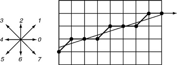
In accordance with our assumption that 0 ≤α ≤ 1, we need to use only the codes 0 and 1. We recall that code 0 is a horizontal increment and code 1 is a diagonal increment; see Figure 9.1.
This definition can easily be adapted to handle straight lines instead of rays. The code sequence of a digital straight line (DSL) is infinite in both directions.
If we use the grid cell model, we can use sequences of grid squares to define digital rays or straight lines:
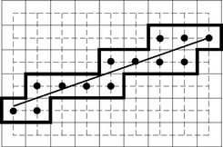
This definition uses the outer Jordan digitization of γ. A cellular straight line segment is defined by a straight line segment γ in the same way. An example is shown in Figure 9.2.
If we translate a cellular straight line by (0.5,0.5) so that its 2-cells are in grid point positions, its frontier consists of two infinite 4-arcs. These 4-arcs can be used to define “upper” and “lower” digital straight lines.
In this introductory section, we present three basic theorems. Theorem 9.1 is about connectivity, which will be treated in Section 9.2; Theorem 9.2 is about self-similarity, which will be treated in Section 9.3; and Theorem 9.3 is about periodicity, which will be treated in Section 9.4.
A finite or infinite 8-arc is called irreducible iff its set of grid points does not remain 8-connected if a nonendpoint is removed from it.
The ray γα,β generates the digital ray iα,β. If β –β′ is an integer, we have iα,β = iα,β′. Thus we can assume without loss of generality that the βs are limited to 0 ≤β ≤ 1. Evidently, i0, β = 000… and i1,β = 111….
Theorem 9.2 If α is irrational, Iα,β uniquely determines both α and β. If α is rational, Iα,β uniquely determines α and determines β up to an interval.
ProofIα,β = α′,β′ implies α = α′, because otherwise the vertical distances between αx +β and α′x+ β′ would not be bounded as x goes to infinity, so the In values would differ beyond some large enough n.
If α is irrational, the values of αx +β modulo 1 for all x ≥ 0 are dense in [0,1]. Hence, for every ε> 0, there exist n0 and m0 such that the following are true, and changing β by ε would result in a change in Iα,β :
Thus Iα,β uniquely determines β when α is irrational.
If α is rational, the set of values of αx +β modulo 1 is finite for x ≥ 0. Hence β is determined only up to an interval with a length that depends on α.
According to Theorem 9.2, iα,β always determines α uniquely. A digital ray is called rational if its slope is rational and irrational if its slope is irrational. For more about the intercepts β, see Section 9.5.
Digital rays are (right) infinite words over {0,1}. We recall a few basic definitions from the theory of words. A (finite) word defined on (or “over”) an alphabet A is a finite sequence of elements of A. The length |u| of the word u = a1a2 …an (where each ai∈ A) is the number n of letters ai in u. The empty word ε has length zero. The set of all words defined on A is denoted by A*1 A word v is a factor of a word u iff there exist words v1 and v2 such that u = v1 vv2. v is a subword of u iff v = a1a2 …an and there exist words v0, v1,…, vn such that u = v0a1v1a2 …anvn.
Let X ⊂ A*. The set of all infinite words w = u0u1u2… (where each ui ∈ X – {ε}) is denoted by Xω. If all of the ujs are equal, for example to v, we write w = vω. For all v ∈ A* and w ∈ Aω, v is a prefix and w a suffix of the concatenation vw.
An integer k ≥ 1 is a period of a word u = a1a2 …an if ai = ai+k (i = 1,…, n – k). The smallest period of u is called the period of u. An infinite word w ε Aω is called periodic if it is of the form w = vω for some nonempty word v ∈ A*. A word w ∈ Aω is eventually periodic if it is of the form w = uvω for some u ∈ A* and some nonempty v ∈ A*. A word w ∈ Aω is called aperiodic if it is not eventually periodic.
The digitization of a ray γα,β in the grid point model is periodic if α is rational and aperiodic if it is irrational:
9.2 Supporting Lines
An alternative way of defining a digital ray is as the 4-border of the upper or lower dichotomy of ![]() 2 defined by a (real) ray. Let the following be true,
2 defined by a (real) ray. Let the following be true,
and let uα,β(n)= Un+1 – Un and lα,β(n)= Ln+1 – Ln. The chain codes uα,β and lα,β are the upper digital ray and lower digital ray generated by γα,β. These upper and lower digital rays are not the same as the grid-intersection digitization of lα,β, but they are also irreducible 8-arcs.
Because Lα,β = Iα,β−0.5, any lower digital ray is also a digital ray and vice versa. If αn +β is not an integer, then Un = Ln + 1. Otherwise, Un = Ln; the digital rays uα,β and lα,β differ in this case, and γα,β has an integral point at n. If γα,β has no integral points, then uα,β = iα,β−0.5 = lα,β. If γα,β has integral points and α is rational, there exists β′ such that Uα,β = Iα,β′. If γα,β has integral points and α is irrational, Uα,β and Lα,β differ by subsequences of length 2 only.
The grid points of a rational ray are the integer solutions of a finite set of linear equations with rational coefficients. Arithmetic geometry2 specifies n-dimensional digital hyperplanes by pairs of linear Diophantine inequalities. In the 2D case, let a and b be relatively prime integers, letμ andω be integers, and let the following be true:
Da,b, μ,ω is called an arithmetic line with slope a/b, approximate intercept μ, and arithmetic width ω [848].
Theorem 9.4 Any set of grid points Da,b,μ,max{|a|,|b|} is the set of grid points of a DSL. Conversely, for any rational DSL, there exist a, b, andμ such that the set of grid points of the given DSL is Da,b,μ,max{|a|,|b|}.
This theorem also implies thatω = max{|a|, |b|} defines an irreducible 8-arc. DSLs are called naive lines in arithmetic geometry, andω = |a| + |b| defines a standard line. See Exercise 9.12 for characterizations of gaps in arithmetic lines. (See Definition 7.13 for definitions of gaps, separation, and gap-freeness.) An arithmetic line is gap-free (8-gap-free) iff it is 4-connected and 4-gap-free iff it is 8-connected. A naive line is 8-connected and 4-separating in Z2, and a standard line is 4-connected and 8-separating in Z2.
Because we are considering only lines with slope 0 ≤ a/(–b) ≤ 1, we have 0 ≤ a ≤–b. For a naive line, we haveω = −b, and all the grid points in Da,b,μ,ω lie between or on two lines ax + by = μ and ax + by = μ – b − 1 (i.e., y = αx +β and y = αx +β – (![]() ) where α = a/– b and β = μ/b). (This proves Corollary 9.1; see p. 314.) These lines are called supporting lines Da,b,μ,ω. (As we will see, supporting lines are used in definitions of DSLs; they are called leaning lines in arithmetic geometry.)
) where α = a/– b and β = μ/b). (This proves Corollary 9.1; see p. 314.) These lines are called supporting lines Da,b,μ,ω. (As we will see, supporting lines are used in definitions of DSLs; they are called leaning lines in arithmetic geometry.)
Digital 4-rays are 4-arcs, where code 2 is a vertical increment:

We can also define upper digital 4-rays ![]() and lower digital 4-rays
and lower digital 4-rays ![]() ; examples are shown in Figure 9.3. We still have
; examples are shown in Figure 9.3. We still have ![]() = 000 …, but we now have
= 000 …, but we now have ![]() = 020202….
= 020202….
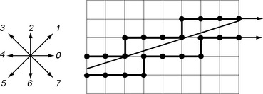
FIGURE 9.3 Segments of lower and upper digital 4-rays that follow the boundaries of the upper and lower dichotomies, which are linearly separated by a ray.
We can define a morphism that maps digital rays into digital 4-rays. A morphism or substitution ϕ : A* → B* is a function such that ϕ(xy) = ϕ(x)ϕ(y) for all x,y ∈ A*.ϕ is uniquely determined by its values for all of the letters in A.ϕ is called nonerasing if it never maps a letter into the empty word. A nonerasing morphism ϕ : A* → B* defines a function (also called a morphism) from Aω to Bω byϕ(a(0)a(1) …a(n) …) = ϕ(a(0))ϕ(a(1)) …ϕ(a(n))…. Digital 4-rays can be defined by the following morphism, which maps digital rays into digital 4-rays:
A chain code is a word over the alphabet {0,…,7} (in our case, {0,1} or {0,2}). Hence, digital rays and DSSs can be regarded as words. In terms of this interpretation, we have the following:
A DSS u connects two points p =(mp, np) and q = (mq, nq) of N2 (mp < mq) iff the geometric interpretation of u = u(1) …u(mq – mp + 1) defines a sequence of horizontal and diagonal steps from p to q. Let u = u(1)u(2) …u(n) be an 8-arc of length n, and let G(u) = {p0, p1,…, pn−1} be the assigned set of grid points such that p0 =(0, 0) and u connects p0 with pn−1 via a sequence of horizontal and diagonal steps through p1,…, pn−2. Theorem 9.4 implies the following:
Theorem 9.5 A finite 4-arc u ?{0,2}* is a 4-DSS iff G(u) lies on or between a pair of parallel lines with a distance apart in the main diagonal direction that is less than ![]() .
.
Proof Letμ be the mapping from {0,1,2}* into {0,1,2}* that is defined by replacing any factor 02 by 1. u ∈{0,1,2}* is a 4-DSS iffμ(u) is a DSS.
Let γ1 and γ2 be parallel lines with a main diagonal distance that is less than ![]() . Consider a finite 4-arc u ∈ {0,2}* such that G(u) lies between or on this pair of parallel lines. If the slope α of these lines is either 0 or 1, u is either 0n or (02)n so that it is a 4-DSS. If 0 <α < 1, we shift the lower line (e.g.,γ2) parallel to itself so it moves closer to γ1 and becomes the lineζ. Then Gμ (u)) lies between or on γ1 andζ, and the distance between them in the y-direction is less than 1, soμ(u) is a DSS and u is a 4-DSS.
. Consider a finite 4-arc u ∈ {0,2}* such that G(u) lies between or on this pair of parallel lines. If the slope α of these lines is either 0 or 1, u is either 0n or (02)n so that it is a 4-DSS. If 0 <α < 1, we shift the lower line (e.g.,γ2) parallel to itself so it moves closer to γ1 and becomes the lineζ. Then Gμ (u)) lies between or on γ1 andζ, and the distance between them in the y-direction is less than 1, soμ(u) is a DSS and u is a 4-DSS.
On the other hand, suppose u ∈ {0,2}* is such that the minimum main diagonal distance between a pair of parallel lines that have G(u) between or on them is at least ![]() . Then u must contain at least one subword 22, soμ(u) is not a DSS and u is not a 4-DSS.
. Then u must contain at least one subword 22, soμ(u) is not a DSS and u is not a 4-DSS.
Two parallel lines at minimum diagonal distance that have G(u) between or on them are called a pair of supporting lines of u. A finite 4-arc is also a finite 8-arc, but lying between or on a pair of parallel lines with a main diagonal distance that is less than ![]() does not imply that the 4-arc is a DSS because it may not be an irreducible 8-arc. A pair of supporting lines with respect to a set Da,b,c,b of grid points has intercepts that differ by 0 < 1 –
does not imply that the 4-arc is a DSS because it may not be an irreducible 8-arc. A pair of supporting lines with respect to a set Da,b,c,b of grid points has intercepts that differ by 0 < 1 – ![]() < 1 so that it has a main diagonal distance of less than
< 1 so that it has a main diagonal distance of less than ![]() .
.
The distance between a pair of parallel lines is measured in the direction of the normal to the lines. Let M be a bounded set in the plane and θ a direction (0 ≤θ < 2π). The width wθ (M) is the minimum distance between a pair of parallel lines such that θ is the direction of the normal to the lines, and M lies between or on them. Let R2×2 be a square formed by four 2-cells.
9.3 Self-Similarity
Self-similarity properties of digital rays and DSSs have been studied in picture analysis. An initial formulation of necessary conditions for self-similarity of DSLs was given by H. Freeman in [344]:
“To summarize, we thus have the following three specific properties which all chains of straight lines must possess [342]:
(F1) at most two types of elements can be present, and these can differ only by unity, modulo eight;
(F2) one of the two element values always occurs singly;
(F3) successive occurrences of the element occurring singly are as uniformly spaced as possible.”
These properties (listed as (1), (2), and (3) in the historic source) were based on heuristic insights and illustrated by examples. Note that property (F3) is not precisely formulated.
9.3.1 The chord property
A. Rosenfeld in [883] gave a first formal characterization of DSLs, which led to a better specification of property (F3).
Theorem 9.7 A finite irreducible 8-arc u ∈ {0,1}* is a DSS iff G(u) satisfies the chord property.
Proof First, we show that G(u) satisfies the chord property if u is a DSS (Theorem 1 in [883]). Let p and q be points of G(u). The line segment pq intersects the grid lines x = n that lie between p and q. Thus, for any point r =(x,y) of pq, we have |n – x|≤ ½ for some point (n, m) ∈ G(u). It suffices to show that, whenever pq crosses a line x = n, the point t = (n, m) of G(u) on that line lies at vertical distance |y – m| < 1 above or below the crossing point r = (n, y).
Let u be a nonempty factor of a digitization of γα,β; then neither p nor q can be more than ½ vertically above γα,β or ½ or more vertically below γα,β. Let r = (n, y) be ar ≥ 0 vertically above γα,β or br ≥ 0 vertically below γα,β. It follows that 0 ≤ ar ≤ ½ or 0 ≤ br < ½. If r is above t,γα,β intersects x = n at vertical distance 0 ≤at < ½ above (or at) t, and we have y – m ≤ ar + at < 1. If r is below t, γα,β intersects x = n at vertical distance 0 ≤ bt ≤ ½ below (or at) t, and we have m – y ≤ br + bt < 1.
Now we prove that u is a DSS if G(u) satisfies the chord property. To do this, we will use the Transversal Theorem of L.A. Santaló (see Section 1.2.8).
Let the 8-arc u join the grid points (n,y0) and (n + m,ym) where m> 0 and ym – y0 ≤ m. If ym – y0 = m, the 8-arc is a diagonal line segment, and the chord property implies that G(u) consists of grid points along this diagonal so that it is a DSS.
Suppose without loss of generality that ym – y0 ≤ m − 1. Let Ti(0 ≤ i ≤ m) be the set of grid points of G(u) on grid line χ = i. The chord property implies that Ti ≠ø and that there are two integers li and ui such that Ti is the set of all grid points (n + i,y) where li ≤ y ≤ ui. Assign a (real) straight line segment L(p) to any grid point p = (x, y), where the following is true:
Let Li be the union of the L(p)s assigned to the grid points of Ti:
Clearly, L0,…, Lm are parallel. Choose any Li, Lj, and Lk (0 ≤ i <j < k ≤ m), and consider two grid points p ∈ Li and q ∈ Lk. The line segment pq intersects the grid line x = j at a point r = (j,yr). By the chord property, there is a grid point t = (xt, yt) ∈ G(u) such that L∞(r,t) < 1. Thus, t is also on x = j (i.e., xt = j). Let s be the midpoint of rt, and let ε = |yt – yr|/2. Let γ be the straight line through s parallel to pq; then 7 intersects x = i at xp ± ε and x = k at xq ± ε. Because ε < 0.5, it follows that γ intersects L(p), L(t), and L(q),so it intersects Li, Lj, and Lk. By the Transversal Theorem, it follows that there exists a straight line γ that intersects all of the Li. It remains only to show that γ generates all of the grid points in G(u) by grid-intersection digitization.
Each Ti contains a grid point pi such that γ intersects L(pi). We have p0 = (n,y0) and pm = (n + m,ym). Let q0 and qm be the intersection points of γ with L(p0) and L(pm) so that q0 = (n,y0 +λ) and qm = (n + m,ym +μ) where −0.5 < λ, μ ≤ 0.5. The horizontal distance between q0 and qm is m, and the vertical distance is |y0 +λ – ym –μ|≤|y0 – ym| + |λ –μ|≤ m − 1 + |λ –μ| < m.
The line segment q0qm makes an angle smaller than 45° with the horizontal direction, so its grid-intersection digitization is specified by intersections with the vertical grid lines x = n + i, 0 ≤ i ≤ m. The grid points produced by these intersections are in G(u), because γ is a transversal of all of the Lis, and G(u) contains only these grid points, because u is an irreducible 8-arc.
Note that infinitely many irreducible two-sided infinite 8-arcs satisfy the chord property but are not digital straight lines (e.g., arcs defined by “sparse” occurrences of 1s in 0ω).
Theorem 9.7 was used in [883] to derive the following necessary conditions on the chain codes of DSSs. These conditions are stated in terms of the runs4 in the chain code.
(R1) “The runs have at most two directions, differing by 45°, and for one of these directions the run length must be 1.
(R2) The runs can have only two lengths, which are consecutive integers.
(R3) One of the runs can occur only once at a time.
(R4) …, for the run length that occurs in runs, these runs can themselves have only two lengths, which are consecutive integers; and so on.”
These properties, which were listed as 1), 2), 3) and 4) in the historic source, do not provide sufficient conditions, but they provide a recursive formulation of (F3).
The chord property is equivalent to a compact chord property that uses the real polygonal arc joining the points of the DSS rather than the real line segment joining its endpoints and the metric L1 rather than L∞.
The property of evenness (“the slope must be the same everywhere”) of a DSS is equivalent to the chord property. “Balance” of words (see Section 9.4) is related to evenness.
9.3.2 Syntactic characterization
Let s = (s(i))i∈I (I ⊆ Z) be a finite or infinite word over N. A letter (in our case, a digit) k is called singular in s iff the following are true:
• for all i ∈ I such that i − 1 and i + 1 are in I, if s(i) = k, then s(i − 1) ≠ k and s(i + 1) ≠ k.
k is nonsingular in s iff it appears in s and is not singular in s. Word s is reducible iff s contains no singular letter or any factor of s that contains only nonsingular letters is of finite length.
Let s be reducible, and let R(s) be the following:
(1) the length of s if s is finite and contains no singular letter;
(2) the word that results from s by replacing by their run lengths all factors of nonsingular letters in s that are between two singular letters in s and deleting all other letters in s; or
Recursive application of this reduction operation R produces a sequence of words s0, s1,… where s0 = s and sn+1 = R(sn). The sequence u0,u1,u2 in Algorithm 9.1 is an example.
Using the DSL property, it is possible to define necessary and sufficient conditions for chain codes of DSSs. Words of nonsingular letters at the ends of the code require special attention. Let s be a finite word, and let l(s) and r(s) be the run lengths of nonsingular letters to the left of the first singular letter and to the right of the last singular letter in s.
L.D. Wu [1137] proved that a chain code has the DSS property iff the corresponding arc is irreducible and has the chord property. This concluded, in 1982, the process of formalizing Freeman’s constraints (F1-F3) and provided a set of constraints on the design of DSS recognition procedures:
A finite factor of a two-sided infinite chain code u satisfies the DSS property iff exactly one straight line defines u by grid-intersection digitization. This implies the following:
9.3.3 Continued fractions
A rational number a1/a0 (a0 > a1 > 0) can be represented by a finite continued fraction with integer coefficients qi > 0(1 ≤ i <n) and qn > 1:

The Euclidean algorithm can be used to derive such continued fractions:

Irrational numbers can be represented by infinite continued fractions.
The value of a continued fraction can be expressed in the following form, where
αn, βn, γn, δn depend on the qis:
For n ≥ 1, we have αnδn −βnγn = (−1)n and the following:
so that the following is true:
Continued fractions can be manipulated using a “concatenation” operator ![]() ; for simple fractions, this operator is defined by (a/b)
; for simple fractions, this operator is defined by (a/b) ![]() (c/d) = (a + b)/(c + d).In terms of
(c/d) = (a + b)/(c + d).In terms of ![]() , we have the following:
, we have the following:

This expression is called the splitting formula in [1107]. The splitting process can continue until only atomic slopes [q] = 1/q remain.
An atomic slope [q] can be encoded by q−1 0s and one 1. Alternating the splitting formulas for odd and even values of n yields a balanced code sequence. For example, 46/87 = [1,1,8,5] gives the following:
This yields the following code sequence, which has length 87 and contains 46 1s:
The splitting formula allows us to express Freeman’s conjecture and Rosenfeld’s recursive process in a very concise way by applying the splitting formula twice, first for n and then for n−1:
(This example assumes that n is even.) This approach handles only DSSs that are factors of rational rays, but we will see in Corollary 9.2 that all DSS shave this property.
9.4 Periodicity
Self-similarity studies have a long history in number theory. The theory of words is a relatively recent discipline that contains many interesting results about self-similarity, often with a focus on irrational straight rays. Rational digital rays are periodic infinite words (Theorem 9.3), and irrational digital rays are a periodic infinite words that are studied under the name of Sturmian words.5 This section gives some basic definitions and results as well as a few proofs.
Let w be a finite or infinite word over A = {0,1}. Let F(w) be the set of all factors of w and Fn (w) the set of factors of w of length n ≥ 0. The complexity function of w is as follows:
P(w, 0) = 1 (the empty word is always a factor), and P(w, 1) is the number of distinct letters in w. For an infinite word w, we have P(w,n) ≤ P(w,n + 1), because every factor of length n can be extended to the right by at least one letter. Furthermore, Fm+n(w) ⊆ Fm(w)Fn(w), so P(w,m + n) ≤ P(w,m) P(w,n).
Let w be an infinite periodic word with period k. Then P(w,n) ≤ k for all n ≥ 0 (i.e., the complexity of a periodic word is limited by its period). The following theorem shows that the converse is also true and generalizes these statements to eventually periodic words. (For example, 10ω is not periodic, but it is eventually periodic, and it is not a rational digital ray.)
A sequence (vn)n≥0 of finite words over an alphabet A converges to an infinite word w if every prefix of w is a prefix of all but a finite number of vn s. For example, the sequence 0n1n converges to 0ω.
Let f1 = 1, f2 = 0, and fn+1 = fnfn−1 for n ≥ 2. The sequence of lengths |fn| is the Fibonacci sequence6 F1 = 1, F2 = 1, F3 = 2, F4 = 3, F5 = 5,…. The sequence (fn)n≥0 converges to the Fibonacci word:
The Fibonacci word can also be defined by a morphism:
Any suffix of a Sturmian word is Sturmian. The Fibonacci word is Sturmian; so is the Thue-Morse word t = μω(0)= 0110100110010110…, where the following are true:![]()
According to Theorem 9.10, any aperiodic infinite word has complexity P(w, n) ≥ n + 1 for n ≥ 0; hence Sturmian words have the least possible complexity. Because a Sturmian word has P(w, 1) = 2, it must be defined on a binary alphabet.
A right special factor of an infinite word w is a finite word u such that u0 and u1 are factors of w. A word w is Sturmian iff it has exactly one right special factor of each length n ≥ 0. (The empty word is the right special factor of length 0.) For the Fibonacci word, 11 is not a factor, so 0 is the only right special factor of length 1; 000 and 011 are not factors, so 10 is the only factor of length 2; and so on.
The height h(w) of a word over {0,1} is the number of 1s in w. If v and w have the same length,δ(v, w) = |h(v) − h(w)| is called their balance. A set X of words is balanced iff |v |= |w| impliesδ(v,w) ≤ 1 for all pairs of words v,w ∈ X. An infinite word w is balanced if its set of factors is balanced.
The slope of a nonempty word w isπ(w) = h(w)/|w|. We have the following:
It can be shown that an infinite word w is balanced iff, for all nonempty factors u and v of w, we have the following:
This shows that the sequence of slopes of w is a Cauchy sequence. Thus a balanced infinite word has a uniquely defined slope that is the limit of the slopes of its finite prefixes. Let w be an infinite balanced word and let wn be the prefix of w of length n ≥ 1. Then the sequence (π(wn))n≥1 converges as n → ∞. For example, for the Fibonacci word f, we have h(fn) = Fn−2 and |fn| = Fn, and Fn−2/Fn converges toπ(f) = 1/τ2 where τ = (1 + ![]() is the golden ratio.
is the golden ratio.
A digital ray is an infinite word that is periodic (aperiodic) iff it is the digitization of a ray of rational (irrational) slope. In the theory of words, digital rays are called mechanical words.
Theorem 9.11 (M. Morse and G.A. Hedlund, 1940) The digitization of a ray of slope α is a balanced word of slope α.
Proof Let w be a lower digital ray. The height of a factor u = w(n) …w(n + p − 1) is h(u)= ![]() α(n + p) +β
α(n + p) +β![]() −
− ![]() αn +β
αn +β![]() . Hence α⋅|u|−1 < h(u) < α⋅|u| + 1 so that
. Hence α⋅|u|−1 < h(u) < α⋅|u| + 1 so that ![]() α⋅ |u|
α⋅ |u|![]() ≤ h(u) ≤ 1 +
≤ h(u) ≤ 1 + ![]() α⋅ |u|
α⋅ |u|![]() . Thus h(u) takes on only two consecutive values when u ranges over factors of w of fixed length, so w is balanced. Moreover, the following is true,
. Thus h(u) takes on only two consecutive values when u ranges over factors of w of fixed length, so w is balanced. Moreover, the following is true,
The inequality |π(u) −α| < 1/|u| provides a criterion for evaluating the accuracy of a slope estimated from a finite DSS. Another method of evaluating the accuracy of an estimated slope will be discussed at the end of Section 9.5.
9.5 Number-Theoretic Properties
9.5.1 Counting segments and partitions
The following theorem is from the theory of words:
It can be shown that a finite word u is balanced iff it is a factor of an irrational digital ray. In accordance with Corollary 9.2, any finite balanced word is also a factor of a rational digital ray (i.e., Theorem 9.13 gives the number of DSSs of length n starting at the origin (0,0)). It is the set of segments u of lower digital rays defined by 0 ≤ x ≤ n,0 ≤α ≤ 1, and 0 ≤β < 1; the first grid point in G(u) is (0,0), and G(u) contains n + 1 grid points. The number of such DSSs that pass through the origin is given as follows:
The Euler function,φ, satisfies the following:
Hence the formula in Theorem 9.13 implies Equation 9.3.
The Farey series F (n) of order n ≥ 1 is the increasing sequence of irreducible fractions between 0 and 1 with denominators that do not exceed n. For example, F(5) is given as follows:
The DSSs of length n that pass through the origin are in one-to-one correspondence with F(n).
There is an obvious one-to-one correspondence between the set of DSSs that start at (0,0) and the set of linear partitions of an n × n grid. (A linear partition of a set S divides it into two parts that are contained in the two halfplanes bounded by a line.) Evidently, any DSS that has n + 1 points and begins at (0,0) defines a linear partition of the n×n grid, but there also exist linear partitions that do not correspond to such DSSs.
The number of linear partitions of an m×n grid (m ≤ n) is given as follows:
This shows how many different digital rays exist on an m×n grid. The asymptotic formulas for the numbers of DSSs and linear partitions can be derived from formulas for average values of number-theoretic functions.
9.5.2 Spirographs
L. Dorst and R. P. W. Duin developed in [278] a theory of spirographs that establishes additional links between digital rays and number theory. Figure 9.4 (left) shows some parallel shifts of a ray with slope α (0 <α < 1) that have y-intercepts in the interval [0,1). For any grid line x = n, there is exactly one grid point (n,yn) such that the ray y = αx +βn passes through (n,yn) and intersects the y-axis in the interval [0,1). Spirographs7 are diagrams that exhibit the distribution of these y-intercepts. As shown in Figure 9.4 (right), the y-intercepts corresponding to rays that pass through grid points (n, yn), n = 0, 1, 2,…, are represented by successive vertices of a (nonsimple) polygon inscribed in a circle of perimeter 1:
Definition 9.8
A spirograph S(α,n) is a set of n points marked on a circle of unit perimeter. The points are the y-intercepts of rays with slope α that intersect the grid lines x = 0, x = 1,…, x = n − 1 at grid point positions.

If α is rational, there are only finitely many such rays, thereby resulting in a finite set of y-intercepts in [0,1) that repeat periodically. The signature of S (α, n) is the order modulo n of the marked points on the circle. (If α is rational, y = αx +β generates the same lower digital ray for all β in an interval; see Theorem 9.2.)
The distance Dα(i,j) between two points i,j ∈ S(α,n), where 0 ≤ i,j < n,is the length of the anticlockwise arc from i to j :

The smallest clockwise distance from 0 ∈ S (α, n) is Dright = min{Dα(i, 0) : i ≠ 0 ∧ i ∈ S(α, n)}. Let the following be the point at this minimum distance:
Similarly, let Dleft = min{Dα (0, i): i ≠ 0 ∧ i ∈ S(α,n) ∧ Dα (0,i) ≠ 0} and the following be true:
By definition, Dright = αright − ![]() αiright
αiright![]() and Dleft = αileft −
and Dleft = αileft −![]() αileft
αileft![]() . Therefore, the bounds on α that preserve the signature of the spirograph are as follows:
. Therefore, the bounds on α that preserve the signature of the spirograph are as follows:
These bounds are the best rational approximations to α using fractions with denominators that do not exceed n − 1. This can be proved from the fact that ![]() αiright
αiright![]() /iright and
/iright and ![]() αiright
αiright![]() /iright are two successive fractions in the Farey series F(n − 1).
/iright are two successive fractions in the Farey series F(n − 1).
For every α (0 ≤α <1) and n (n ≥ 1), there is an interval of possible intercepts β (0 ≤β < 1) such that the given lower straight line segment of length n is a digitization of the ray αx +β. The width of this interval defines the maximal possible error Emax(α,n); see Figure 9.5. Emax, (α,n) is the maximum arc length in the spirograph S(α,n):
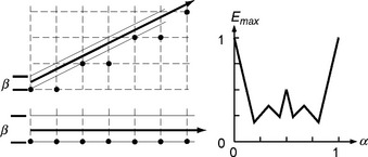
FIGURE 9.5 Left: the maximum error inß as a function of the estimated α value for n = 6 [278]. Right: the maximum error inß is 1 for α = 0 and 05 for α = 0.5.
The formula Dright + Dleft = ![]() αileft
αileft![]() −
− ![]() αiright
αiright![]() +α(iright − ileft) using the values from S(α,n + 1) provides a simple method of calculating the errors εmax(α,n). If α is a fraction a/b in the Farey series F(n), then Emax(a/b,n) = 1/b.
+α(iright − ileft) using the values from S(α,n + 1) provides a simple method of calculating the errors εmax(α,n). If α is a fraction a/b in the Farey series F(n), then Emax(a/b,n) = 1/b.
9.6 Algorithms
Many efficient DSS recognition algorithms have been published. The computational problem is as follows: the input is a sequence of chain codes i(0),i(1),… where i(k)∈ {0,1} and k ≥ 0. An offline DSS recognition algorithm decides whether a finite word u ∈{0, 1} * is a DSS. An online DSS recognition algorithm reads the successive chain codes i(0),i(1),… and determines the maximum k ≥ 0 such that i(0),i(1),…, i(k) is a DSS but i(0),…,i(k),i(k + 1) is not. A recognition algorithm has linear run time behavior (is a linear algorithm) if it runs in O(n) time (i.e., it performs at most O(|u|) computation steps for any finite input word u ∈ {0,1}*). Analogous definitions can be given for 4-DSS recognition algorithms. An online algorithm is linear if it uses on the average a constant number of operations for each input chain code symbol.
9.6.1 Design paradigms
The decomposition of a 4- or 8-arc into a sequence of DSSs or 4-DSSs is a more general computational problem that includes DSS or 4-DSS recognition as a subproblem. Obviously a linear online DSS recognition algorithm supports a linear decomposition algorithm, but linear offline algorithms allow only quadratic runtime behavior.
The design of a DSS recognition algorithm may be based on a particular characterization of DSSs, such as the following:
(C1) the original definition of a DSS based on grid-intersection digitization;
(C2) a characterization by pairs of supporting lines (e.g., (C2.1a) Theorem 9.4, (C2.1b) Corollary 9.1, (C2.2) Theorem 9.5, (C2.3) Theorem 9.6);
(C3) the equivalence with the chord property (see Theorem 9.7); and
(C4) the DSS property (see Theorem 9.8).
Algorithms that use (C4) are often called linguistic techniques.
9.6.2 A linear online DSS recognition algorithm
We review in detail one of the first linear online DSS recognition algorithms, published in 1982 in [223], which uses (C4).
Algorithm CHW 1982a
The input sequence is u = i(0)i(1)i(2) …i(n), i(k) ε A = {0,1,…,7},0 ≤ k ≤ n. Let u0 = u, and, if uk−1 ≠ε (the empty word), let uk = R(uk−1) where R is the reduction operation used in Section 9.3 to define the DSL and DSS properties. Let l(k) and r(k) be the run lengths of nonsingular letters to the left of the first singular letter in uk or to the right of the last singular letter; see Definition 9.6
The input sequence is u = i(0)i(1)i(2) …i(n), i(k) ∈ A = {0,1,…,7},0 ≤ k ≤ n. Let u0 = u, and, if uk−1 ≠ε (the empty word), let uk = R(uk−1) where R is the reduction operation used in Section 9.3 to define the DSL and DSS properties. Let l(k) and r(k) be the run lengths of nonsingular letters to the left of the first singular letter in uk or to the right of the last singular letter; see Definition 9.6. Let s(k) be the singular letter in uk if there is one or −1 otherwise. Let n(k) be the second letter in uk if there is one or −1 otherwise. Algorithm 9.1 shows an example. The input chain code u0 is now represented by a syntactic code, which is as follows for the given example:
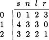
In general, the code consists of integers in four columns s, n, l, and r. The DSS property (see Definition 9.6) imposes constraints on these integers so that the given
word u = i(0)i(1)i(2) …i(n) can be classified as being a DSS or not. Before starting to read a word, initialize the values in columns s and n to −1 and the values in columns l and r to 0. Suppose the syntactic code has been calculated for an input sequence of length ≥ 0 and the next input chain code is d. Let N(k, a, b) be true iff |a − b| = 1 for k ≥ 1 and | a − b | (modulo 8) = 1 for k = 0. The algorithm uses tests that follow straightforwardly from the DSS property:
The algorithm inserts new elements d into the code of Algorithm 9.1 as long as the incoming chain code satisfies the DSS property.
Algorithm CHW1982a runs in linear time: |uk+1|≤ ½ ·|uk| for all k ≥ 0 and any input DSS chain code. There is only one loop in the algorithm in the case in which a new element needs to be added to one of the uks. Therefore its run time t(n) for inputs of length n =|u0| is on the order of the following:
It also follows that the number of relevant integers in the syntactic code is at most O (log n), because the index m of the last nonempty word um satisfies m ≤ log2n. A stronger inequality is as follows:
For example, n = 2377… 5739 requires only reduced chain code words uk for k ≤ m = 9. Of course, representing a DSS by the endpoints of one of its possible preimages is an even shorter representation.
9.6.3 Review of other algorithms
This section briefly reviews some other DSS recognition algorithms and details an algorithm that segments an 8-arc into maximum-length DSSs.
Algorithm CHW1982b
Our second linear online algorithm, published in [223], uses the set of possible preimages (see approach (C1)); as long as this set is nonempty, we can continue to read chain code symbols.
Let the DSS u ε {0, 1}* of length n connect grid point p0 =(0,0) with grid point pn through grid points p1,…, pn−1. Let −0.5 ≤ lx ≤ ux < n + 0.5 be segments of the grid lines x = 0, x = 1,…, x = n, which are the unions of all intersections of these grid lines, with possible straight line segment preimages of u with respect to grid-intersection digitization, so that x − 0.5 ≤ lx ≤ ux < x + 0.5. Note that segment (x, lx)(x,ux) may degenerate into a single point (i.e., lx = ux). Segment (x, lx)(x,ux) must not contain the grid point px (0 ≤ x ≤ n); see Figure 9.6. The sequence of points (0,u0), (1, u1),…, (n, un), (n,ln), (n − 1, ln−1),…, (0,l0) is called the digitization polygon of u. Because (x, lx)(x,ux) may degenerate into a single point, the digitization polygon need not be simple. Note that the segments (0, u0)(n,ln) and (0,l0)(n,un) are contained in the digitization polygon.

Let u be extended by adding another chain code a ∈ {0,1}. The 8-arc ua is a DSS iff it has a digitization polygon. The linear online algorithm CHW1982b, described in detail in [223] and also published in [222], uses the digitization polygon of u to construct the polygon for ua if possible or returns “no” if there is no polygon for ua.
The digitization polygon of a DSS is the union of all of the line segments with digitization that is the given DSS. Digitization polygons were also studied in [279]. Any DSS is uniquely characterized by a quadruple of integers: its length, its shortest period, its lowest-terms slope, and its phase. From this quadruple, we can calculate the digitization polygon.
Algorithm S1983
[988] gives a linguistic technique (see (C4)) for segmenting an 8-arc into DSSs. As in CHW1982a, this algorithm involves only integer operations using the syntactic rules specified in the DSS property. A parser checks the rules related to each layer k and (eventually) activates a parser for the next layer k + 1. Several parsers at different layers may be active simultaneously. The maximum number of layers is bounded by 4.785·log10n + 1·672 and is taken on for digital rays of slopes a/b where a and b are consecutive Fibonacci numbers [566]. The average number of layers is less than half of this value [566].
[988] reports on experiments that compared polygons with vertices that are the break points of segmented 8-arcs with the polygonal preimages of these 8-arcs with respect to grid-intersection digitization. It describes an ambiguity in defining maximum-length DSSs defined by these break points.
Algorithm AK1985
[20] has already been cited in connection with pairs of supporting lines for 8-arcs; it gives a DSS recognition algorithm that follows approach (C2.1b). Let u ∈ {0,1}* be an 8-arc of length n connecting grid point p0 =(0,0) with grid point pn through grid points p1,…, pn−1. Critical points are a minimal subset of G(u) = {p0, p1,…, pn} that defines a pair of supporting lines that have a minimum distance in the y direction and that have G(u) between or on them. An 8-arc u is a DSS iff this distance is < 1; see Corollary 9.1.
Without loss of generality, let u have four critical points q1, q2, r1, r2 ∈ G(u) where q1q2 specify a nearest support below u and r1r2 a nearest support above u. Then u is uniquely specified either by n and q1,q2 or by n and r1,r2. [20] describes a linear offline algorithm for calculating the nearest support below and/or above u. A final test (Corollary 9.1) decides whether or not u is a DSS. This algorithm has also been used to define a linear offline algorithm for calculating the digitization polygon (see algorithm CHW1982b). [20] also discusses the calculation of digitization polyhedra for DSSs in 3D space.
Algorithm CHS1988a
[222] gives three linear online DSS recognition algorithms. The first is a slightly improved version of algorithm CHW1982b. The second also uses approach (C1); however, this time the definition of grid-intersection digitization is used to perform DSS recognition by solving a separability problem for a monotonic polygon.
Let u ∈ {0,1}* be an 8-arc of length n connecting grid point p0 = (0,0) with grid point pn through grid points p1,…, pn−1. Let pk = (k,Ik), k = 0,1,…, n. The weak digitization polygon of u is defined by vertices (0,I0 + 0.5), + 0.5),…, (n,In + 0.5), (n, In − 0.5), (n − 1, In−1 − 0.5),…, (0, I0 − 0.5). This polygon is monotonic in the x direction. The separability problem is as follows: u is a DSS iff the upper polygonal chain (0, I0 + 0.5), + 0.5),…, (n,In + 0.5) of its weak digitization polygon can be separated from its lower polygonal chain (n, In − 0.5), (n − 1, In−1 − 0.5),…, (0, I0 − 0.5) by a straight line that does not intersect either polygonal chain. [222] gives a linear online algorithm for solving this separability problem for ua based on a solution for u. The separability problem can also be stated as the problem of determining the visibility of (0,I0 − 0.5)(0,I0 + 0.5) from (n, In − 0.5)(n, In + 0.5) or vice versa.
Algorithm CHS1988b
The third linear online DSS recognition algorithm in [222] uses (C2.1b). It is similar to (but independent of) the linear offline algorithm AK1985. It uses the critical points calculated for u to calculate critical points for ua if possible and returns “no” otherwise. The algorithm is quite short and allows a quick implementation. [222] also contains a geometric analysis of possible and impossible locations of critical points. If a critical point of u is cancelled in an extended uv, it cannot become a critical point in extensions of uv.
Algorithm SD1991
[1007] discusses a linear offline DSS recognition algorithm that uses the linguistic approach (C4). It begins with Wu’s linear offline algorithm [1137] and corrects the flaw described in [454].
Algorithm DR1995
[256] describes a linear online DSS recognition algorithm that uses the (C2.1a) approach; the naive line in [256] is the same as a DSL (see the comment following Theorem 9.4). The algorithm is based on updating two linear Diophantine inequalities, which amount to a test of whether G(u) is in a strip (see algorithm K1990)of width max{|a|, |b|}. For details of this algorithm, see Chapter 11, where it is used for 3D DSS recognition.
9.6.4 A linear online 4-DSS algorithm
[592] discusses the recognition of 4-DSSs on the frontier of a region in a 2D incidence grid using approach (C2.3). Because this algorithm is one of the simplest and most efficient linear online 4-DSS recognition algorithms, we will give it in full detail. It is based on the calculation of a narrowest strip defined by the nearest support below and above (see Theorem 9.5). It resembles the linear offline algorithm AK1985 and the linear online algorithm CHS1988b for 8-arcs. For the notation, see Figure 9.7; for examples, see Figure 9.6.4.
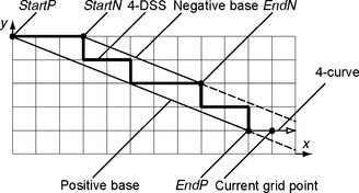
FIGURE 9.7 [592] Notation for algorithm K1990.
Algorithm K1990
This algorithm follows a digital 4-curve and extends a 4-DSS as long as it has at most two directions and all of its grid points lie between or on a pair of parallel lines that have a main diagonal distance of less than ![]() . On the parallel line to the left of the digital curve, we define a negative base between the grid points pN = StartN and qN = EndN, and, on the parallel line to the right of the digital curve, we define a positive base between the grid points pP = StartP and qP = EndP.
. On the parallel line to the left of the digital curve, we define a negative base between the grid points pN = StartN and qN = EndN, and, on the parallel line to the right of the digital curve, we define a positive base between the grid points pP = StartP and qP = EndP.
A sequence of grid points (x, y) on the digital 4-curve is a 4-DSS iff the following is true,
where (a, b)T is a vector v parallel to the negative (or positive) base of the 4-DSS that has relatively prime integer coordinates and c is an integer (constant for the 4-DSS) such that c = ay − bx for any grid point (x, y) on the negative base. Let h(x,y) = bx − ay + c, and suppose the inequalities are true for n − 1 accepted grid points of the 4-DSS. When a new 4-DSS is initialized, let the first step be from p = (x1, y1) to the 4-adjacent q = (x2, y2); let pN := qP :=p, qN :=Pp := q, a := x2 − x1, b : = y2 − y1, and note the direction of the step from p to q. Whenever a new step is not in one of the (at most two) directions in the current 4-DSS, we start a new DSS. When there has been only one direction so far, we continue the current DSS. If there have been two directions, we consider the cases shown in Algorithm 9.3.
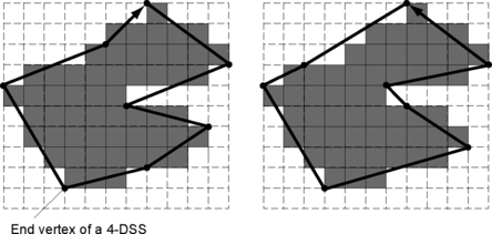
Note that in case (iii), we have a new vector v that defines new values a, b, and c. In cases (i) and (ii), we have to move either qN or qP forward into position rn. Figure 9.8 illustrates a clockwise and an anticlockwise traversal of the frontier of a digital region that produce different segmentations into maximum-length 4-DSSs.
9.7 Exercises
1. Segment the infinite word w = 01102103 …0n 10n + 1… into a sequence of consecutive DSSs of maximum lengths.
2. Consider the “spiral” in Z2 that starts at the origin o = (0,0) and is represented by the infinite chain code w = 01 1234 …nn + 1… = 0112223333…. Let un = 0 13 …nn + 1 be a prefix of w that defines a path from o to pn. Characterize the asymptotic growth of the Euclidean distance de(o,pn). Is this growth linear, quadratic, polynomial of order m, or exponential?
3. Prove Equation 9.2 for infinite words w.
4. Let F(iα,β) be the set of all factors of the DSL iα,β. Prove that F(iα,β) = F(iα,0) for any irrational α.
5. Let iα,β and iα,β2 be DSLs with the same rational slope α. Prove that there exists an m ∈ ![]() such that iα,β1 (n) = iα,β2 (n + m) for all n ∈ Z.
such that iα,β1 (n) = iα,β2 (n + m) for all n ∈ Z.
6. Let G be the set of grid points of a DSS, and let C(G) be the Euclidean convex hull of G (see Chapter 13). Prove that the points of G are the only grid points in C(G).
7. Two DSSs are called parallel (perpendicular) iff they are grid-intersection digitizations of parallel (perpendicular) straight line segments. Show that there exists a simply connected 4-region G that is not the set of grid points contained in a rectangle but with a 4-border that consists of two mutually perpendicular pairs of parallel DSSs.
8. Let Um(p) = {q ∈ Z2 : d8(q,p) ≤ m} where m ≥ 0. We say that an 8-arcπ has the skeleton property iff, for any distinct p and q in G(p) and any point r on the (real) line segment pq, there exists a grid point t ∈ G(p) such that max{d8 (r, s): s ∈ Um(t)} < m + 1. Prove that an 8-arc has the chord property iff it has the skeleton property.
9. Let Gp,q be the set of all grid points that are on DSSs that connect p with q. Show that Gp,q is an 8-region and that the 4-border of Gp,q can be segmented into at most two DSSs.
10. Algorithms CHW1982a and K1990 both have O(n) run time complexity (say f (n) = an + b with a,b > 0) on DSSs of length n (nL ≤ n ≤ nU). Estimate a and b for each algorithm.
11. Give an example of a simple 8-curve and an initial point such that the numbers of DSSs in a segmentation of the curve into maximum-length DSSs are different for a clockwise and a counterclockwise traversal of the curve.
12. Let Da,b,μ,ω = {(i,j)∈ Z2 :μ ≤ ai + bj <μ +ω} be an arithmetic line, where a and b are relatively prime integers such that 0 ≤ a ≤ b andμ andω are integers. Prove the following:
(i) D is 8-disconnected (i.e., D has 4-gaps; see Definition 7.13 ifω < b).
9.8 Commented Bibliography
The computer representation of lines and curves has been an active subject of research for nearly half a century [121, 342, 342, 883]. Related work even earlier on the theory of words [748] (specifically on mechanical or Sturmian words) remained unnoticed in the pattern recognition community. The material on the theory of words cited in this chapter follows [667, 668].
Theorem 9.1 is from [883]. For Theorem 9.2, see [140]. It has been known since [137] that grid-intersection digitization of rays γα,β produces periodic digital rays if α is rational and aperiodic digital rays if it is irrational (Theorem 9.3). An algorithm for “symmetric grid-intersection digitization” that does not depend on the clockwise or counterclockwise orientation of the curve is given in [1052]. [137] gives an algorithm for calculating the basic segment of a rational digital ray for β = 0. [1137] gives an algorithm for calculating the basic segment of such a ray using α and β as inputs.
The grid points of a rational ray are the integer solutions of a finite set of linear equations with rational coefficients [101]. This property was of basic importance for the establishment of arithmetic geometry [332, [848]]. Theorem 9.4 and Exercise 12 are from [848].
Corollary 9.1 was proved in [30] using the chord property of Theorem 9.7; see also [20, 222].
[140,312,592] used digital 4-rays instead of 8-rays. [312] introduced digital rays in the grid cell model; sequences of bordering 1-cells define 4-rays. Digital 4-rays can also be generated by global mappings defined on digital 8-rays. The geometric characterization of 4-DSSs is discussed in [592] based on results in [20] about the “nearest support below or above” of a DSS.
Theorem 9.5 is an unproved statement in [592]. For Theorem 9.6, see [312].
An early algorithm for generating a DSS that connects two arbitrary grid points p and q was published in [843]. [137] proposed grammars for chain code generation of rational digital rays based on Freeman’s criteria (F1), (F2), and (F3).
Theorem 9.7 was proved in [883]. The proof given in Section 9.3.1 that u is a DSS if G(u) satisfies the chord property is from [864]. Alternative proofs of some of the results in [883] (at most two run lengths that are successive integers and one of which occurs only as singletons) are given in [348]. The compact chord property is discussed in [978]. A variant of the chord property for the outer Jordan digitization of a straight line segment was given in [867]. The chord property and its generalization to a chordal triangle property for Z3 are discussed in [866]. The property of evenness is studied in [454]. In [456], it is proved that the absence of runs that differ by more than 1 is equivalent to the chord property. [454] calls nonbalanced words uneven and proves that an infinite 8-arc has the chord property iff it has no uneven finite factors.
[528] gives three necessary and sufficient conditions (detailed definitions omitted here) for a digital arc to be a DSS: (i) its total absolute curvature is 0; (ii) its width in some direction is 0; and (iii) its length in some direction is less than half of the perimeter of its convex hull.
It has also been proved that point sequences generated by (a version of) Brons’ parallel algorithm have the chord property [30, 31]. The formal language L of DSSs is context-sensitive; see [316] and later publications [802, 931, 1138]. This implies that linear-bounded or cellular automata can recognize DSSs using “string rewriting rules.” A result in the theory of words [288] says that the complement {0,1}*/L of the set of all DSSs is a context-free language.
Definition 9.5 is a precise formulation of criteria (F1-F3); it is used in [451] to define a DSS algorithm. The given formulation follows [449]. Definition 9.6 and Theorem 9.9 are also from [449].
[1136] does not contain the important algorithm published in [1137]. Regarding Theorem 9.8, [1137] does not contain a theorem but only statements about an algorithm specified by a flow chart. However, it is easily seen that this algorithm is actually an implementation of the DSS property as described above, so [1137] actually contains a proof of Theorem 9.8, including the generation of straight lines that have rational or irrational slopes. [1137] also considers the case of an infinite code sequence and shows that any finite factor of a two-sided infinite chain code c has the DSS property iff exactly one straight line with slope α and intercept β defines c by grid-intersection digitization.
Material for a concise proof of Wu’s theorem based on properties of Farey series was published in [278] in the form of an algorithm.8 Proofs of Wu’s theorem based on continued fractions (see Section 9.3.3) were published in 1991 in [140, 1105]; see also [1107]. The use of continued fractions to model digital rays was discussed in [137]. Related results in number theory [464] have been useful in these studies. We reviewed related definitions from number theory and reported results given by K. Voss in [1107].
For the theory of words, see [667, 668]. The definition of “Sturmian words” follows [668]. Some authors use the name “Sturmian words” for lower DSLs; see, for example, [74]. The proof of Theorem 9.10 (from [219]) is a citation of the proof of Theorem 1.3.13 in [668] as given by J. Berstel and P. Séébold. Theorems 9.11 and 9.12 are from [748]. The proof of Theorem 9.11 is a citation of the proof of Lemma 2.1.14 in [668] as given by J. Berstel and P. Séébold. Periodicity studies of digital rays can also be based on signal-theoretic (Fourier transform) methods (see [635]); this allows characterization of approximate periodicity.
Theorem 9.13 is from [728]. Asymptotic estimates of the number of DSSs of length n are given in [73]. [74] gives another proof of Theorem 9.13 and also an algorithm for random generation of lower DSSs of length n. Equation 3 is from [585]. [656] contains earlier related work. [653] uses the author’s results on the number of DSSs in an n × n grid to show that piecewise DSS coding of digital curves requires O(n4) table entries.
Suggestions about using Farey series to model digitized lines were made in [137, 274, 332, 738, 931]. In [931], it is shown that DSSs of length n through the origin are in one-to-one correspondence with the nth Farey series. The number of linear partitions of an m × n orthogonal grid is considered in [4] (Equation 4). Theorem 9.14 is from [279]. See [1099] for a more recent discussion about Farey numbers for characterizing DSLs.
Linear offline algorithms for DSS recognition based on the DSS property (see Definition 9.6) were published in 1981 in [451] and in 1982 in [1137].9 A linear offline algorithm for cellular straight segment recognition based on convex hull construction is briefly sketched in [517,509]. In [516], it is shown that a digital set is digitally convex iff the border digital arcs between the vertices of its convex hull are DSSs. A finite set of lattice points that lie between two lines at unit min (horizontal, vertical) distance is a DSS. A digital arc is a DSS iff it is convex. Convexity will be treated in Chapter 13.
The extended abstract [515] discusses digital arcs and digital convexity: a digital arc is a DSS iff it has the chord property; a digital set is digitally convex iff the convex hull of its set of corner points contains no corner point of its complement; and a digital arc is a DSS iff it is digitally convex (this is proved for several definitions of digitization in [516]). These conditions can be checked in linear offline time using run length coding. Algorithms in [516] deal with determining whether a digital region is a digital convex polygon.
Two linear online algorithms for DSS recognition were published in 1982 by E. Creutzburg, A. Hübler, and V. Wedler [223]; one of them is an online version of the offline algorithm published in [451]. For an early version of a linguistic DSS recognition algorithm, see [931]. (It was not based on the correct DSS property, which became known later.)
The general problem of decomposing a 4- or 8-arc into a sequence of 4-DSSs or DSSs, which includes 4-DSS or DSS recognition as a subproblem, is discussed in, among others, [256, 542, 542, 1007].
Many DSS recognition algorithms have not been reviewed here due to space limitations (e.g., [175, 341, 601, 650, 654, 655, 912, 990, 1155]). The original source of algorithm K1990 is [592]; see also [542, 593] for discussions of this algorithm. A method of segmentation into a minimum number of DSSs in linear time based on calculating a tangential representation is given in [324]. Segmentation into “fuzzy DSSs” (defined using arithmetic geometry) is discussed in [254]. Scattering of points away from a “true” DSS is considered in [159].
Section 10.3 will describe performance evaluations of a few DSS recognition algorithms. Still lacking is a comprehensive and comparative evaluation of such algorithms. A statistic analysis of empiric time complexities would also be of interest. The random DSS generation algorithm of [74] could be used to create input data.
The segmentation of an 8-curve into maximum-length DSSs (see [223]) depends on the starting point and orientation of the traversal of the curve. It would be of interest to analyze the possible variation in such segmentations.
Different adjacency definitions may be worth studying in greater detail in connection with DSS algorithms; see, for example, [699] about digitizations in a 16-neighborhood. Straightness in 3D or higher-dimensional digital spaces would also be worth studying. (See, for example, [1028]: a set of grid points is an n-dimensional DSS iff n − 1 of its projections onto the coordinate planes are 2D DSSs.) Finally, straightness can be discussed in multivalued digital pictures. (In [529], positional errors are estimated for straight edges between regions that have given constant values as a function of the size of the picture and its number of values.)
Exercises 4 and 5 are from [675]. For Exercise 6, see [516]. Exercise 7 is from [599]. Parallel DSSs are studied in [812]. Exercise 8 is from [979], and Exercise 9 from [811]. For other references about digitized straight lines, see [174, 280, 382,722].
1A* was also used in the definition of dimension, but the context will always clarify the meaning.
2See also Chapter 11.
4A run is a maximum-length factor an of a word.
5[748] introduced the term Sturmian trajectories after the mathematician C.F. Sturm (1803–1855), who is famous for his rule for computing the roots of an algebraic equation. [748] defined Sturmian words as zeros of solutions of linear homogeneous second-order differential equations.
6Standard notation as used in The Fibonacci Quarterly.
7This was named after a children’s toy that is used for drawing curves.
8The DSL property is called “linearity conditions” in [278]. See also our discussion of [278] in Section 9.5.