
Incidence Pseudographs
This chapter treats pictures as graph-theoretic objects; it represents spatial subdivisions with incidence pseudographs. We recall that, in 2D or 3D incidence grids (see Section 2.1.5), pixels or voxels are further refined (e.g., a 2-cell [grid square] has grid edges and grid vertices as additional structural components). We define open and closed subsets of incidence pseudographs and their frontiers in preparation for discussing topologies in the following chapters. We give combinatorial formulas for such subsets in regular incidence grids and give a graph-theoretic treatment of frontier tracing.
5.1 Incidence Structures
In this chapter, we discuss a graph-theoretic generalization of the grid cell incidence model (see Section 2.1.5). Because self-incidence is allowed, the graphs can have loops (i.e., they are pseudographs).
Let I be a reflexive and symmetric relation on a set S. We say that c and c′ are incident (notation: cIc′) iff {c, c′} ∈ I.
The function dim partitions S into pairwise disjoint classes. Its definition depends on the context. For example, the elements of S can be cells of a discrete spatial subdivision (e.g., convex bounded polyhedra or polygons, line segments, vertices); Figure 5.1 shows a 2D example. A cell c that has dim(c) = i is called an i-cell. Such spatial subdivisions are studied in combinatorial topology. In 1813, A. Cauchy generalized the Descartes-Euler polyhedron theorem by studying intercellular faces in simple polyhedra. Finite or infinite 2D or 3D incidence grids (see Section 2.1.5)—or subsets of such grids that form 2D or 3D regions—are other examples of discrete spatial subdivisions.

FIGURE 5.1 Left: geometric representation of the incidence structure of the Voronoi diagram shown in Figure 4.3. Middle: a substructure. Right: its graph; loops are omitted, and labels give the dimensions of the Voronoi cells, edges, and vertices.
Incidence pseudographs provide a method of describing discrete spatial subdivisions by local relations. In this section, we formulate the general n-dimensional case to illustrate potential generalizations, but our main focus continues to be on 2D and 3D grids.
5.1.1 Adjacency and completeness; incidence pseudographs
Let G =[S,I, dim] be an incidence structure. c ∈ S is called an i-node if dim(c) = i. The maximum value of dim(c) for any c ∈ S is called the index dimension ind(G) of G.1 If ind (G)= n, G is called an n-incidence structure. Any node of G that has dimension ind(G) is called a principal node, and any node that has smaller dimension is called a marginal node.
For example, 2D and 3D incidence grids define incidence structures ![]() and
and ![]() of index dimensions 2 and 3, respectively, in which pixels and voxels are the principal nodes. We generalize the adjacency definitions given for incidence grids in Section 2.2.1. Let I(c) = {c′ : c′ ∈ S Λ c′Ic}.
of index dimensions 2 and 3, respectively, in which pixels and voxels are the principal nodes. We generalize the adjacency definitions given for incidence grids in Section 2.2.1. Let I(c) = {c′ : c′ ∈ S Λ c′Ic}.
A relation Ai of i-adjacency between nodes of an incidence structure defines an adjacency structure Gi = [S, Ai], which is an adjacency graph if properties A1 through A3 are satisfied. All of the definitions and results regarding adjacency graphs in Chapter 4 apply to these Gis. For example (see Definition 4.1), two nodes c, c′ ∈ S are i-connected with respect to M ⊆ S iff there is an i-path (c1, c2,…, ck) in [S, I, dim] where c = c1, c′ = ck, and the nodes of the path are either all in M or all in ![]() This allows us to define i-components of M.
This allows us to define i-components of M.
Figure 5.1 (middle or right) shows (on the upper left) that, unlike the situation for adjacency grids, i-adjacency of two nodes does not necessarily imply h-adjacency for h <i.
This (symmetric and irreflexive) adjacency relation defines paths of nodes of equal dimension j > 0, and the reflexive and transitive closure of this relation defines connectedness and components for such nodes. Components of an incidence structure will be defined in the next section; these components need not contain only nodes of a single dimension.
Our main interest is in principal nodes. Let G =[S, I, dim] be an n-incidence structure. The set of n-nodes of G is called the core of G. G is called an incidence pseudograph iff it has the following properties:
I1: For any node c of G, I(c) is finite.
I2: The core of G is connected.
I3: Any finite set of principal nodes of G has at most one infinite complementary component of principal nodes.
I4: If c′ ∈ I(c) and c′ ≠ c, then dim(c′) ≠ dim(c).
I5: Any marginal node of G is incident with at least one principal node of G.
Properties I1 through I5 are independent of one another. This is easy to verify; see Section 4.1.3. Figure 5.2 shows a finite incidence pseudograph with core {a, e, f}.

FIGURE 5.2 An incidence pseudograph with nodes a,…, f. The dimensions of the nodes are indicated by the labels.
An incidence pseudograph is called monotonic (short for “in transitive correspondence with a monotonic chain of dimensions”) iff the following is true:
I6: If c′ ∈ I(c) and c" ∈ I(c′), where dim(c) ≤ dim(c′) ≤ dim(c′′), then c″ ∈ I(c). For example, the pseudograph in Figure 5.2 is not monotonic because, for example, c ∈ I(b) and b ∈ I (a) but ![]() Properties I4 and I6 indicate that the incidence corresponds to a partial order relation on S: c < c′ iff c and c′ are incident and dim(c) < dim(c′). This allows us to define a poset topology; see Section 6.1.2.
Properties I4 and I6 indicate that the incidence corresponds to a partial order relation on S: c < c′ iff c and c′ are incident and dim(c) < dim(c′). This allows us to define a poset topology; see Section 6.1.2.
Finally, we generalize Definition 2.5 (completeness) from incidence grids to arbitrary incidence pseudographs. Let G =[S, I, dim] be an incidence pseudograph, and let M ⊆ S. We define the completion M + of M with respect to G as the smallest subset of S that has the following properties:
Property (ii) leads to a recursive procedure for adding nodes: first (ind(G) −1)-nodes, then (ind(G) − 2)-nodes, and so forth. Figure 5.3 shows a rectangular subset of the 2D incidence grid2 that is completed by adding six 1-nodes and then adding three 0-nodes.

FIGURE 5.3 Left: a set M that has four 1-components of 2-nodes. Right: its completion M +, which has two 1-components of 2-nodes (loops omitted).
Figure 5.1 (middle) is an example of a complete subset.
The core of the subset M on the left in Figure 5.3 is connected; it consists of four 1-components of 2-nodes. M is a proper subset of M +, so M is not complete; the core of M + contains two 1-components of 2-nodes.
5.1.2 Incidence grids
[S, I, dim] is called a 2D or 3D incidence grid iff one of the following is true: (i) it is ![]() or
or ![]() ; (ii) it is a finite complete subpseudograph of
; (ii) it is a finite complete subpseudograph of ![]() defined by a core that is an m × n rectangular subset of
defined by a core that is an m × n rectangular subset of ![]() ; or (iii) it is a finite complete subpseudograph of
; or (iii) it is a finite complete subpseudograph of ![]() defined by a core that is an l × m × n cuboidal subset of
defined by a core that is an l × m × n cuboidal subset of ![]() .
.
Any incidence grid has properties I1 through I6, as well as two other properties:
I7: If c ∈ S and dim(c) > 0, there is a c′ ∈ S such that dim(c′) < dim(c) and {c,c′} ∈ I.
I8: If cIc′ and dim(c) – dim(c′) > 1, there is a c″ ∈ S such that dim(c′) < dim(c″) < dim(c), cIc″, and c′Ic″.
In addition, the nodes of an incidence grid have locations in Euclidean space. Incidence grids are the “default examples” of incidence pseudographs, just as α- or (α1,α2)-adjacency grids are the “default examples” of adjacency graphs.
The cores of incidence grids are sets of pixels (2-cells) or voxels (3-cells). Definition 5.2 allows two 1-cells of ![]() to be 0-, 2-, or 3-adjacent, but, in accordance with property I4, they cannot be 1-adjacent. A 1-path in
to be 0-, 2-, or 3-adjacent, but, in accordance with property I4, they cannot be 1-adjacent. A 1-path in ![]() can contain 0-, 2-, or 3-cells but not 1-cells. An i-path or i-component can be restricted to contain only cells of a given dimension; see Figure 2.18. A path of cells of dimension i is defined by 0-, 1-,…,or (i − 1)-adjacency.
can contain 0-, 2-, or 3-cells but not 1-cells. An i-path or i-component can be restricted to contain only cells of a given dimension; see Figure 2.18. A path of cells of dimension i is defined by 0-, 1-,…,or (i − 1)-adjacency.
Example 5.1
Any adjacency graph G =[S, A] can be represented by a one-dimensional incidence pseudograph GI with a set of nodes that is S ![]() A. Elements of S have dimension 0, and elements of A have dimension 1. Every c ∈ A is incident with its two endnodes in S, and every c ∈ S is incident with all of the edges {c, c′} in A. Every node of GI is also self-incident.
A. Elements of S have dimension 0, and elements of A have dimension 1. Every c ∈ A is incident with its two endnodes in S, and every c ∈ S is incident with all of the edges {c, c′} in A. Every node of GI is also self-incident.
Figure 5.4 shows the one-dimensional incidence pseudograph of ![]() . Repeated merging operations (contraction; see Section 4.2.2), as shown in the middle of Figure 5.4 (including the deletion of all loops), can be used to transform this graph into a graph isomorphic to
. Repeated merging operations (contraction; see Section 4.2.2), as shown in the middle of Figure 5.4 (including the deletion of all loops), can be used to transform this graph into a graph isomorphic to ![]() .
.

FIGURE 5.4 The one-dimensional incidence pseudograph of the 1-adjacency grid (left; all loops are omitted). Two merging operations are illustrated: a 1-node merges with a 0-node (middle); a 0-node merges with a 1-node (right).
Let G =[S, I, dim] be an n-incidence grid (n ≥ 1), and let 0 ≤ n0 < n. By deleting all i-nodes from S (n0 < i ≤ n) and all edges that have these i-nodes as endnodes, we obtain an n0-incidence pseudograph that is a subpseudograph of [S, I, dim]. Such a subpseudograph is called a downward restriction of G For example, let G be the 3D incidence grid ![]() , and let n0 = 2. We can delete all 3-cubes from
, and let n0 = 2. We can delete all 3-cubes from ![]() to obtain a subpseudograph that consists of only grid squares, grid edges, and grid vertices. Figure 5.5 shows a 2D example: a one-dimensional downward restriction of a rectangular subgraph of
to obtain a subpseudograph that consists of only grid squares, grid edges, and grid vertices. Figure 5.5 shows a 2D example: a one-dimensional downward restriction of a rectangular subgraph of ![]() , which can be transformed into
, which can be transformed into ![]() by repeated merging operations.
by repeated merging operations.

FIGURE 5.5 A 2D incidence grid, its downward restriction (both without loops), and a contraction of the downward restriction.
A finite nonempty complete subset M ⊆ S of an incidence grid [S, I, dim] defines an incidence structure [M, I′, dim′], where I′ and dim′ are the restrictions of I and dim to M. Such a structure satisfies properties I1 through I3 but need not satisfy properties I4 through I8.
5.1.3 Components and regions; borders
In this section, M is a complete subset of an n-incidence structure G =[S, I, dim].
For example, M + on the right in Figure 5.3 is a component. A nonempty M may have no components, and the union of all of the components of M may not be all of M. Even a complete M is not always a union of components; there may be i-nodes in M (i < n) that are not incident with any n-node of M. Our main interest is in finite M s that are unions of components.
The following definitions are analogous to the definitions for adjacency graphs in Section 4.1.3:
For example, the incidence pseudograph shown in Figure 5.2 is a region. The completion of its core {a, e, f} is {a, d, e, f}. {a, b, d, e, f} and {a, c, d, e, f} are regions. M + on the right in Figure 5.3 is a region, but M on the left is not a region, because it is not complete.
Definition 5.7
A node c (of any dimension) of a region M is called an inner node iff I (c) ⊆ M; otherwise, it is called a border node. The set of inner nodes of M is called the inner set ![]() of M, and the set of border nodes of M is called the border δM of M.
of M, and the set of border nodes of M is called the border δM of M.
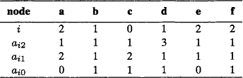
If M = S, it has only inner nodes. Figure 5.6 shows two examples of inner sets and borders. (Closed and open regions will be defined in the next section.) The same sets are shown in Figure 5.7 using the geometric representation of 2D incidence grids that was defined in Section 2.1.5.

FIGURE 5.6 Inner sets (bold unfilled circles) and borders (bold filled circles) of a closed (left) and an open (right) region. The left region remains closed after deleting 2-node a; this deletion creates an open hole.

FIGURE 5.7 Geometric representations of the regions shown in Figure 5.6 Label a identifies the same 2-node as in Figure 5.6.
5.1.4 Closed and open regions
The following definitions do not have analogs for adjacency graphs:
Definition 5.8
A subset M ⊆ S of an incidence structure G =[S,I, dim] is called closed in G iff, for any c ∈ M and any c′∈ I(c) such that dim(c’) < dim(c), we have C′ ∈ M. M is called open in G iff ![]() is closed in G.
is closed in G.
Figure 5.6 shows examples of a closed and an open region. In Figure 5.2, {a, d, e, f} is an open region, because {b,c} is a closed set (but not a region); {a,b,d,e,f} is open; and {a, c, d, e, f} is neither closed nor open. In Figure 5.3, M + on the right is neither closed nor open. Evidently, S and θ are both closed and open. Any closed or open M is complete. Closed and open sets are not necessarily components; they may contain only nodes of dimensions < n, or they may be disconnected.
The proof of Proposition 2.3 gave a procedure for assigning every 0- or 1-cell of the 2D incidence grid to exactly one incident 2-cell in a 2D picture P, and Proposition 2.4 generalized this procedure to the 3D incidence grid. The procedure was based on a decomposition of the grid into P-equivalence classes, which define incidence substructures that are unions of components (and hence are complete). These substructures, except for the one that contains the infinite background component, are all finite. Figure 5.8 shows an example in which the 2D procedure produces either “black closed components” and “white open components” or vice versa.

FIGURE 5.8 The black pixels (left), shown as a closed (middle) and an open (right) region of the 2D incidence grid.
As a direct consequence of the definition of closedness, we have the following:
Theorem 5.3
A finite subset M ⊆ S of an n-incidence pseudograph G =[S,I, dim] is an open region in G iff the core of M is nonempty and connected, and (B) an i-cell ![]() (i <n) is in M iff every j-cell c′ such that cIc′ and i <j ≤ n is in M. If G is monotonic, M is an open region in G iff its core is nonempty and connected, and (C) an i-cell
(i <n) is in M iff every j-cell c′ such that cIc′ and i <j ≤ n is in M. If G is monotonic, M is an open region in G iff its core is nonempty and connected, and (C) an i-cell ![]() is in M iff all of the n-cells in I(c) are also in M.
is in M iff all of the n-cells in I(c) are also in M.
Proof The complement of an open set is closed; (B) is the complementary formulation of (A) in Theorem 5.2. (C) uses only the n-cells in I (c), but (B) uses all of the j-cells in I(c) such that i <j ≤ n so that (B) implies (C). Let M satisfy (C), let the i-cell c be in M, and suppose there exists a j-cell c′∈ I (c),i <j ≤ n such that ![]() . Then at least one n-cell in I(c′) is not in M and hence is not in I(c), which is impossible if G is monotonic.
. Then at least one n-cell in I(c′) is not in M and hence is not in I(c), which is impossible if G is monotonic.
The incidence pseudographs in Figures 5.3 and 5.6 are monotonic.
The closure ![]() of a finite subset M of an n-incidence pseudograph is the smallest closed region that contains M. We can construct the closure of M by adding all cells c′ such that c′ ∈ I(c) and dim(c′) < dim(c) for some c ∈ M.
of a finite subset M of an n-incidence pseudograph is the smallest closed region that contains M. We can construct the closure of M by adding all cells c′ such that c′ ∈ I(c) and dim(c′) < dim(c) for some c ∈ M.
5.2 Boundaries, Frontiers, and the Euler Characteristic
5.2.1 Boundaries, chains, and frontiers
Let G =[S, I, dim] be an n-incidence pseudograph. A node c ∈ S is invalid with respect to M ⊆ S iff ![]() , but there is an n-node c′ ∈ M such that c′∈ I (c). This definition generalizes the concepts of invalid edges and boundaries in adjacency grids. We recall that any adjacency graph can be transformed into a one-dimensional incidence pseudograph; see Example 5.1.
, but there is an n-node c′ ∈ M such that c′∈ I (c). This definition generalizes the concepts of invalid edges and boundaries in adjacency grids. We recall that any adjacency graph can be transformed into a one-dimensional incidence pseudograph; see Example 5.1.
Figure 5.9shows two examples of boundaries for n = 2. The boundary of S is empty, and the boundary of a region contains no principal nodes.

FIGURE 5.9 Two regions (bold, unfilled circles) and their boundaries (bold, shaded circles). Left: closed region. Right: open region.
Let M ⊂ S be finite. A cell c of M will be denoted by c(i) if dim(c) = i. An i-chain is an expression of the form C(i) = ![]() where each bk = 0 or 1 and the sum is taken over all of the i-dimensional cells of M. We say that
where each bk = 0 or 1 and the sum is taken over all of the i-dimensional cells of M. We say that ![]() is in C(i) iff bk = 1; we can identify C(i) with the set of i-nodes that are in C(i). We define the addition of i-chains modulo 2:
is in C(i) iff bk = 1; we can identify C(i) with the set of i-nodes that are in C(i). We define the addition of i-chains modulo 2: ![]() where the bs are added modulo 2. Thus
where the bs are added modulo 2. Thus ![]() is in the sum of two i-chains iff it is in exactly one of the chains. We write C(i) = 0 if all of its bs are 0 so that it corresponds to an empty set of i-nodes.
is in the sum of two i-chains iff it is in exactly one of the chains. We write C(i) = 0 if all of its bs are 0 so that it corresponds to an empty set of i-nodes.
Let C(i) be an i-chain (i> 0). The chain frontier ![]() is the (i − 1)-chain
is the (i − 1)-chain ![]() where ak is the number (modulo 2) of i-cells in C(i) that are incident with C(i−1). For i = 0, we define
where ak is the number (modulo 2) of i-cells in C(i) that are incident with C(i−1). For i = 0, we define ![]() = 0. It is not hard to show that
= 0. It is not hard to show that ![]() is a linear operator (i.e.,
is a linear operator (i.e.,![]() [modulo 2]).
[modulo 2]).
C(i) is called an i-cycle if ![]() = 0. Evidently, a 0-chain is a cycle; a sum of i-cycles is an i-cycle; and the frontier of any chain is a cycle (i.e., for any i-chain, we have
= 0. Evidently, a 0-chain is a cycle; a sum of i-cycles is an i-cycle; and the frontier of any chain is a cycle (i.e., for any i-chain, we have ![]() ).
).
Figure 5.10 shows a subset M of the 2D incidence grid, with 2-cells abhg, bcih, and so on; 1-cells ag, ab, and so on; and 0-cells a, b, and so on. Using the above definitions, we have ![]() a = 0;
a = 0; ![]() ab = a + b;
ab = a + b; ![]() abgh = ab + bh + gh + ag;
abgh = ab + bh + gh + ag; ![]() (ij + jn + no + ko + jk) = i + 3j + 2n + 2o + 2k = i + j; and jk + ko + no + jn is a 1-cycle.
(ij + jn + no + ko + jk) = i + 3j + 2n + 2o + 2k = i + j; and jk + ko + no + jn is a 1-cycle.

For example, the open region A consisting of the single 2-node jkno in Figure 5.10 has boundary M = {j, k, n, o, jk, ko, no, jn}. The set of 1-nodes in M has an empty frontier, so it is a 1-cycle.
Let M be a closed region in an infinite incidence pseudograph. ![]() is the union of a finite number of pairwise disjoint open regions and one infinite open subset of S. A (finite) open region is either an open hole (if it is circumscribed by its boundary) or an open finite background region; the infinite open subset is the open background. The border nodes of the closed region in Figure 5.11 are shown in Figure 5.12. If we assume that the incidence pseudograph in Figure 5.11 is a subset of the 2D incidence grid and use nodes of the incidence grid not shown in the figures, the border also contains the two 1-nodes in the top row and three more 1-nodes and five more 0-nodes that “close” the border on the right and at the bottom.
is the union of a finite number of pairwise disjoint open regions and one infinite open subset of S. A (finite) open region is either an open hole (if it is circumscribed by its boundary) or an open finite background region; the infinite open subset is the open background. The border nodes of the closed region in Figure 5.11 are shown in Figure 5.12. If we assume that the incidence pseudograph in Figure 5.11 is a subset of the 2D incidence grid and use nodes of the incidence grid not shown in the figures, the border also contains the two 1-nodes in the top row and three more 1-nodes and five more 0-nodes that “close” the border on the right and at the bottom.

FIGURE 5.11 A closed region in an infinite incidence pseudograph (a “stripe” bounded on the right and unbounded on the left) that has three open holes (in the 1-adjacency graph of 2-nodes, two of these would be improper holes and one a proper hole), three open finite background regions, and an (infinite) open background.

FIGURE 5.12 Boundary nodes of the closed region shown in Figure 5.11.
Similarly, if M is an open region, we obtain closed holes (circumscribed by their borders), closed finite background regions, and a closed background. Figure 5.6 (or Figure 5.7) shows an open hole (after removing node a), and Figure 5.13 shows an open region for which the infinite background is a closed component (but not a region because it is infinite). The boundary nodes in Figure 5.14 coincide with the boundary nodes of the open region in Figure 5.13.

FIGURE 5.13 An open region that has one closed hole (in the 1-adjacency graph of 2-nodes this would be a proper hole), three closed finite background regions, and an (infinite) closed background component with a core that consists of three 1-components.

FIGURE 5.14 Boundary nodes of the complementary open regions of the closed region shown in Figure 5.11.
Theorem 5.2
If the closed component M1 is the closure of the open component M2, the border of M1 coincides with the boundary of M2.
Proof The border δM1 of a closed component M1 consists of all nodes c for which c ∈ M1 and I(c)![]() M1.c cannot be a principal node, because M1 is closed so that I (c′) ⊂ M1 for any principal node c′; however, c is incident with at least one principal node in M1 because of Definition 5.5. It follows that the nodes of δM1 constitute the boundary of the open set M1δM1.
M1.c cannot be a principal node, because M1 is closed so that I (c′) ⊂ M1 for any principal node c′; however, c is incident with at least one principal node in M1 because of Definition 5.5. It follows that the nodes of δM1 constitute the boundary of the open set M1δM1.
Node c is in the boundary of an open component M2 iff c∉M2, but there exists a principal node c’ ∈ M2 such that c’ ∈ I (c). It follows that all boundary nodes of M2 are in the closure ![]() of M2, hence in the border of this closed component. Conversely, let c be in the border of
of M2, hence in the border of this closed component. Conversely, let c be in the border of ![]() ; because M2 is a component, c is incident with a principal node of M2, so c is in the boundary of M2.
; because M2 is a component, c is incident with a principal node of M2, so c is in the boundary of M2.
We recall Definition 3.2 for a subset A of a Euclidean space: the frontier ![]() A is the set-theoretic difference between the closure A• and the interior A°. The frontier of A°,of A•, or of any set containing A° and contained in A• is also
A is the set-theoretic difference between the closure A• and the interior A°. The frontier of A°,of A•, or of any set containing A° and contained in A• is also ![]() A.
A.
Definition 5.11
Let M ⊆ S be a subset of an incidence structure G =[S, I, dim]. The frontier ![]() M of M is the border of M•.
M of M is the border of M•.
In analogy with the Euclidean topology, we call ![]() the interior of M. Note that, if M is a component, M° is an open component.
the interior of M. Note that, if M is a component, M° is an open component.
Section 4.3.6 discussed borders and boundaries in adjacency grids at the abstract level of adjacency graphs. There we were able to state alternatives, but were unable to unify “border” and “boundary” as in Theorem 5.2, which led to Definition 5.11.
5.2.2 The matching theorem
The matching theorem in this section is a basic combinatorial formula for finite incidence pseudographs of index dimension n ≥ 0.
Definition 5.12
Let G =[S, I, dim] be an incidence pseudograph, and let c ∈ S. The number shown here is called the incidence count of c:
Because of self-incidence and property I4 (see Section 5.1.1), if dim(c) = i, we have aii(c) = 1. Table 5.1 gives examples of incidence counts.
Theorem 5.2
Proof If i ≠ j, all of the edges between i-nodes and j-nodes (and only those edges) are counted in the sum; see Figure 5.15. All edges are undirected, and the number of endpoints in both sums is the same. If i = j, the sum is equal to the number of i-nodes.

Equation 4.4 follows from the matching theorem, because v(p) = a01(p) for any node p of an adjacency graph [S, A]. Equation 4.4 can also be derived using the incidence counts a10(e) for the edges e:
This definition generalizes Definition 4.7. The complete graphs Kn are examples of finite regular one-dimensional incidence pseudographs. The nodes of Kn have dimension 0, the edges of Kn have dimension 1, and every node is self-incident. The infinite incidence grids ![]() and
and ![]() are also regular.
are also regular.
If G has index dimension n ≥ 1 and M is a finite subset of G, the numbers shown here are called the class cardinalities of M:
We usually omit the superscript M.
From the Matching Theorem, we know that, for finite regular incidence pseudographs, we have αiaij = αjaji for 0 ≤ i, j ≤ n. It follows that this equation holds true
for any (e.g., fixed) index k (0 ≤ k ≤ n). Hence the possible integer values of the class cardinalities αk and αi define constraints (Diophantine equations) on the incidence counts aki and aik (and vice versa).
5.2.3 The Euler characteristic
In this section, we generalize the definition given in Section 4.3.2 for finite oriented adjacency graphs in 2D. Note that an edge is incident with a cycle iff it is listed in the cycle, and a node is incident with an edge iff it is one of the edge’s endnodes.
Definition 5.14
Let G =[S,I, dim] be a finite n-incidence pseudograph (n ≥ 1). The Euler characteristic of G is as follows, where the αis are the class cardinalities of S:![]()
For example, for the G shown in Figure 5.2, we have x(G) = 1 − 2 + 3 = 2. Adding an edge (e.g., between nodes b and e) does not change the Euler characteristic. However, deleting a node (e.g., 2-node e) results in an incidence pseudograph G′ for which x(G′’) = 1 −2 + 2 = 1.
If G is regular, the Matching Theorem gives us the following:
These n + 1 equations (k = 0, 1,…, n) are rational multiples of one another.
Figure 5.16 shows regions in the infinite regular incidence grid ![]() that define subpseudographs (loops omitted). For the upper left region, we have χ = 3 − 10 + 8 = 1; for the lower left region, we have x = 1 − 4 + 4 = 1; for the region on their right, we have χ = 5 − 5 + 1 = 1; and, for the remaining 1-path, we have χ = 7 − 6 + 0 = 1. For the region M + shown on the right in Figure 5.3, we have χ = 15 − 28 + 14 = 1; note that removing marginal border nodes changes this value. In Figure 5.6, for the closed region on the left, we have χ = 12 − 33 + 22 = 1, and, for the open region on the right, we have χ = 12 − 15 + 4 = 1. Removing the “central” 2-node a from the closed region creates an “open hole” and gives χ = 11 − 33 + 22 = 0. These examples illustrate the topologic invariance of the Euler characteristic; see Section 6.4.5.
that define subpseudographs (loops omitted). For the upper left region, we have χ = 3 − 10 + 8 = 1; for the lower left region, we have x = 1 − 4 + 4 = 1; for the region on their right, we have χ = 5 − 5 + 1 = 1; and, for the remaining 1-path, we have χ = 7 − 6 + 0 = 1. For the region M + shown on the right in Figure 5.3, we have χ = 15 − 28 + 14 = 1; note that removing marginal border nodes changes this value. In Figure 5.6, for the closed region on the left, we have χ = 12 − 33 + 22 = 1, and, for the open region on the right, we have χ = 12 − 15 + 4 = 1. Removing the “central” 2-node a from the closed region creates an “open hole” and gives χ = 11 − 33 + 22 = 0. These examples illustrate the topologic invariance of the Euler characteristic; see Section 6.4.5.

5.3 The Regular Case
An incidence pseudograph provides a more “refined” representation of a grid than does an adjacency graph representation. We begin by discussing regular infinite incidence pseudographs defined in ![]() , but as usual, the cases of interest involve incidence relations on finite or countable sets of 0-, 1-, 2-, or 3-cells.
, but as usual, the cases of interest involve incidence relations on finite or countable sets of 0-, 1-, 2-, or 3-cells.
5.3.1 Regular infinite incidence pseudographs
The incidence grids ![]() and
and ![]() , when regarded as pseudographs [S, I, dim], are monotonic (property I6) and also have properties I7 and I8.
, when regarded as pseudographs [S, I, dim], are monotonic (property I6) and also have properties I7 and I8.
Definition 5.15
The set of all 0-cells is the set (0.5,…,0.5) + ![]() . Let c be a k-cell in a k-dimensional subspace of
. Let c be a k-cell in a k-dimensional subspace of ![]() (0 ≤ k ≤ n). Let ej be the straight line segment with endpoints that are the origin o and the point (0,…,0,1,0,…, 0) where the 1 is in position j (1 ≤ j ≤ n). Let ej be in an n – k dimensional subspace of
(0 ≤ k ≤ n). Let ej be the straight line segment with endpoints that are the origin o and the point (0,…,0,1,0,…, 0) where the 1 is in position j (1 ≤ j ≤ n). Let ej be in an n – k dimensional subspace of ![]() . The Minkowski sum c
. The Minkowski sum c ![]() ej in
ej in ![]() defines a (k + 1) -cell. The set of all i-cells is denoted by
defines a (k + 1) -cell. The set of all i-cells is denoted by ![]() , and the union of the
, and the union of the ![]() is denoted by
is denoted by ![]() .
.
This generalizes Definition 2.1. An informal description is as follows: A 1-cell is “created” by translating a 0-cell along any of the segments ej. A 2-cell is the area occupied by a 1-cell while it shifts along an orthogonal segment ej, and a 3-cell is the volume occupied by a 2-cell while it shifts along an orthogonal segment ej. Figure 5.17 illustrates these processes up to the creation of a 4-cell.

FIGURE 5.17 Examples of how a Minkowski sum (“union during translation along an orthogonal line segment ej”) of an i-cell creates an (i + 1)-cell.
![]() (n ≥ 1) is called the regular n-incidence grid. It can be verified that it has properties I6 and I8. Its incidence counts are as follows:
(n ≥ 1) is called the regular n-incidence grid. It can be verified that it has properties I6 and I8. Its incidence counts are as follows:
For example, an i-cell c ∈ ![]() is incident with 2n–1 n-cells. Equation 5.3 implies the following for 0 ≤ i, j ≤ n:
is incident with 2n–1 n-cells. Equation 5.3 implies the following for 0 ≤ i, j ≤ n:

Equation 5.4 in turn implies the following for 0 ≤ i ≤ n:

5.3.2 The region matching theorem
In this section, ![]() are class cardinalities, and aij are incidence counts in the regular incidence grid
are class cardinalities, and aij are incidence counts in the regular incidence grid ![]() . Note that the aij are constants. For n = 2, they are as follows:
. Note that the aij are constants. For n = 2, they are as follows:
For n = 3, they are as follows:
a00 = 1, a01 = 6,a02 = 12, a03 = 8,
a10 = 2, a11 = 1, a12 = 4,a13 = 4,
a20 = 4, a21 = 4, a22 = 1,a23 = 2,
a30 = 8, a31 = 12, a32 = 6,a33 = 1
The numbers shown here are called boundary counts for the cells in M:

The numbers shown here are called total boundary counts for M:
From now on, we omit the superscript M.
Theorem 5.2
(the Region Matching Theorem): Let M be an open or closed region in the regular incidence grid ![]() . For 0 ≤ i, j ≤ n, we have the following:
. For 0 ≤ i, j ≤ n, we have the following:
αiaij – bij = αj aji for i <j if M is closed or for i>j if M is open
αiaij + bji = αjaji for i>j if M is closed or for i <j if M is open.
Proof Let M be closed. In the equations for i <j, the right sides are the number of j-cells in M times the number of i-cells that are incident with any of these j-cells (i.e., the number T of incidences between j -cells in M and i-cells). All of these i-cells are also elements of M; see (A) in Theorem 5.2. The total number of incidences between i-cells in M and j-cells in M is evidently T. However, the i-cells in M are also incident with bij j-cells, which are not in M; hence the count αiaij on the left side of the equation must be reduced by bij.
The second equation is trivial and is given only for completeness.
The equations for j <i are proved for a closed region M by simply swapping i and j in the discussion of the i <j case. For an open region M, we use (B) from Theorem 5.3.
Note that the proof of this theorem makes no use of the connectedness of a region, but only of its being either closed or open. Figure 5.18 shows an open and a closed region. For the open region, we have α0 = 0,α1 = 1,α2 = 2, b10 = 2, b20 = 8, and b21 = 6; for example, 1 · 2 + 6 = 2 · 4 if i = 1 and j = 2. For the closed region, we have α0 = 7,α1 = 8,α2 = 2, b01 = 12, b02 = 20, and b12 = 8; for example, 7 · 4 − 20 = 2 · 4 if i = 0 and j = 2.

The formulas of the Region Matching Theorem hold for any finite union of pairwise disjoint closed (or open) regions.
For a closed region M or a finite union of pairwise disjoint closed regions, the Region Matching Theorem implies the following:

For example,αn specifies the contents of an isothetic polyhedron in ![]() (n ≥ 2). These formulas allow us to calculate αn based on counts of, for example, vertices; see Section 8.1.6 for n = 2 and Section 8.3.7 for n = 3. Using Equation 5.5, it follows that the Euler characteristic, as follows,
(n ≥ 2). These formulas allow us to calculate αn based on counts of, for example, vertices; see Section 8.1.6 for n = 2 and Section 8.3.7 for n = 3. Using Equation 5.5, it follows that the Euler characteristic, as follows,

can be calculated for any j (0 ≤ j ≤ n) by counting only invalid cells (cells on the boundary of the region). Similarly, for an open region M or a finite union of pairwise disjoint open regions, we have the following for any 0 ≤ j ≤ n:
Indices j = 0 and j = n give the simplest expressions. In the next section, we will show that these expressions can be further simplified.
5.3.3 Euler characteristics
We apply the Region Matching Theorem and Conclusion 5.3.2:
Lemma 5.1 Let M be a finite union of pairwise disjoint closed regions in the n-incidence grid. For 0 ≤ i, j ≤ n, we have the following:
Proof The proof is by downward induction starting at i = n:
Assuming that the equation is correct for i ≥ 1, we show that it is also correct for i − 1. From the Region Matching Theorem, for a closed region we have the following, where Equation 5.4 can be used to simplify products of b-values:

Analogously, for open regions, we have the following:
Lemma 5.2 Let M be a finite union of pairwise disjoint open regions in the n-incidence grid. For 0 ≤ i, j ≤ n, we have the following:

The following theorem was proved by K. Voss in 1993 for open regions:
Theorem 5.2 Let M be a finite union of pairwise disjoint closed (or open) regions in ![]() . Then the Euler characteristic of M is as follows:
. Then the Euler characteristic of M is as follows:![]()
and![]()
Proof We prove the theorem for open regions; closed regions can be treated analogously. Lemma 5.2 and the equation ![]() show that the following is true:
show that the following is true:

The double sum can be rearranged: first take the sum for all j-values and then for all i-values. It follows that what is shown here is true:

The formula for closed regions then follows from Equation 5.4 and for 0 ≤ m <n:

The bi–1,is and bi+1,i s in Theorem 5.2 can be replaced with class cardinalities and (globally known) incidence counts because the following are given:
Let n = 3. For a closed region, b01 is the number of invalid grid edges incident with grid vertices in the region, b12 is the number of invalid grid squares incident with grid edges in the region, and b23 is the number of invalid grid cubes incident with grid squares in the region. For open regions, we use b10, which is the number of invalid grid vertices incident with grid edges in the region; b21, the number of invalid grid edges incident with grid squares in the region; and b32, the number of invalid grid squares incident with grid cubes in the region. Note that the total boundary counts are sums over all cells in M so that invalid cells may be counted repeatedly if they are incident with several cells in M.
Figure 5.19 shows a 2D example. For the left closed region, we have b12 = 16 and b01 = 16, and, for the right closed region, we have b12 = 4 and b01 = 8. For the left open region, we have b21 = 16 and b10 = 16, and, for the right open region (a single node), we have b21 = 4 and b10 = 0.

5.4 Pictures on Incidence Grids
In a labeled incidence pseudograph G =[S, I, dim], each node in G has a label, and the labels belong to a finite set {L0,…, Lmax}.
A picture assigns labels (values of pixels or voxels) to all of the principal nodes of S. We assume that the set of these labels is totally ordered by “significance,” so nodes labeled Lmax are the “most significant” (e.g., “object pixels”) and nodes labeled L0 are the “least significant” (e.g., “background pixels”). For example, a 2D picture assigns labels (pixel values) to all 2-cells in G m,n and label L0 to all 2-cells in the infinite background component.
An ordered labeling of the nodes of an incidence pseudograph is defined by assigning labels to the principal nodes and extending this labeling to the other nodes by applying the following maximum-label rule:
According to I5, any marginal node has candidate labels, and, according to I1, the set of candidates is finite, which allows us to choose the largest of them. The rule ensures that regions labeled with Lmax are closed and regions labeled with L0 are open.
In picture processing or analysis, we do not need to perform actual labeling but only to detect adjacencies between labeled principal nodes, assuming that all marginal nodes have been labeled. During a scan through the set of principal nodes, we have to decide whether two nodes c1 and c2 such that I(c1) ∩ I(c2) ≠ ø are still adjacent after ordered labeling. An algorithm for this is given in Algorithm 5.1. An order by decreasing node dimension (Step 2) has been assumed for efficiency reasons; the scan through the marginal nodes in I(c1) ∩ I(c2) should visit nodes with I(c) s that have increasing cardinalities, and the ordering by node dimension may ensure this.
If G is a binary picture and we assume that black (or white) is the most significant label, the resulting adjacency is just the (4,8)- or (8,4)-adjacency defined in Section 2.1.4. These two adjacencies are illustrated in Figure 5.20, together with the corresponding representations of the components in the incidence grid.

FIGURE 5.20 (4,8)- and (8,4)-adjacencies and the corresponding representations of the components in the incidence grid.
The situation is more complicated if G is a multilevel picture, because there are many possible total orderings of the labels. Figure 5.21 illustrates three such orderings for a three-valued picture; each ordering yields a different adjacency structure.

FIGURE 5.21 A three-valued input picture (from left to right): all of the 4-components in the grid point model; closed (open) regions are black (gray); closed (open) regions are gray (white); closed (open) regions are gray (black).
In the next section, we will describe a general method of defining adjacencies for a given ordered labeling. In a 2D picture, this method yields adjacencies in which diagonal adjacencies never “cross,” as illustrated in Figure 5.22. These adjacencies can be defined using the 2 × 2 masks shown in Figure 5.23. Note that these masks accept all 4-adjacencies between pixels that have the same label and that they also accept diagonal adjacencies between two pixels that have the same label as a third pixel that is adjacent to both of them. Only in case (g) is it necessary to choose between
ALGORITHM 5.1 Local adjacency decision procedure, assuming an ordered labeling.

FIGURE 5.22 Left: the binary picture from Figure 1.10. Right: adjacencies resulting from ordered labeling, assuming “white is less significant than black” and dropping crossing pairs of diagonals.

tween the (black, black) and (white, white) diagonal adjacencies. When this method of defining adjacencies is used, the adjacencies define a planar graph, and, as we will see in Chapter 7, the resulting region adjacency graph is a tree.
5.4.2 The ordered adjacency procedure
We now describe a general procedure for the ordered labeling of incidence grids that applies in particular to 2D or 3D multilevel pictures. Let G =[S, I, dim] be a labeled n-incidence grid, and assume a total ordering of the set of labels. Our ordered adjacency procedure defines adjacencies between principal nodes of G that depend on this total order.
Let S be finite, let c0 be a 0-cell, and let I (n)(c0) be the set of all principal nodes in I(c0). We begin with any 0-cell c0 in S and any pair c1 and c2 of nodes in I (n)(c0), and we proceed as described in Algorithm 5.2. We then continue for all of the remaining 0-cells in S.
This procedure guarantees that components are defined by (n − 1)-adjacency between principal nodes if they have the same label or by i-adjacency (i <n) if their label “wins” over at least one “competing” label. It simplifies the switch approach described in Section 2.1.3 by eliminating redundant adjacencies and generalizes it to incidence grids of arbitrary dimension.
The result of applying the procedure to the multilevel picture shown in Figure 2.19 is shown in Figure 5.24. The scan of I(n)(c0) to list all pairs (c1,c2) in it can be based on a uniform local cyclic order, but the result is independent of the order in which the pairs are chosen.

FIGURE 5.24 Ordered adjacencies for the picture shown in Figure 2.19 assuming the same order of the picture values as in Figure 2.19.
The adjacency defined by applying the procedure to a picture depends only on the total order of the labels 0,…, Gmax. As a default, we assume the order 0 < 1 < … <Gmax, for which we have the following:
5.4.3 Frontiers in 2D incidence grids
In a 2D incidence grid, the boundary of a closed region consists of one or more 1-components of 2-cells (grid squares), and the boundary of an open region consists of one or more 0-components of 1-cells (grid edges). The union of the 1-cells in the boundary of an open region is the same as the boundary of the region in the 1-adjacency grid. Figure 4.27 (right) shows an example.
The set of 1-cells that are incident with exactly one 2-cell of a region defines the frontier of the region. Every 0-component of these 1-cells has a Hamiltonian circuit that visits each 1-cell in the 0-component exactly once.3 The border tracing algorithm (see Chapter 4) can be used to trace the border cycles in the 0-adjacency graph of these 1-cells.
We now describe a method of representing these sets of 0- and 1-cells. Let P be a picture on an m × n grid G, which we call the picture grid. We extend this grid to an (m + 1) × (n + 1) frontier grid F, where each grid point in F represents a grid vertex (0-cell) in F specifically, grid vertex (x–0·5, y−0·5) in G represents grid point (x,y) in F4 Figure 5.25 shows the picture grid and the frontier grid for the picture shown in Figures 1.10 and 5.22.
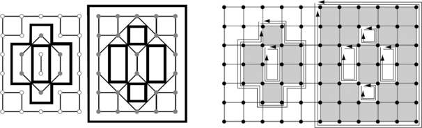
FIGURE 5.25 Left: picture grid showing the ordered adjacencies and frontiers for all components. Right: frontier grid showing the Hamiltonian circuits for all 0-components of 1-cells of all frontiers.
The geometric representation of the frontiers in G is the union of the small squares and thin rectangles that represent 0-cells and 1-cells, respectively. Figure 5.25 shows counterclockwise frontier traversals for the interior regions and clockwise traversals for the exterior regions and the (infinite) background component. This reflects the use of local circular order (A) in Figure 4.19. We use the following notation when q2 is the direct successor of q1 in the local circular order at pi :![]()
To traverse all of the frontiers, we scan the picture (e.g., using a standard scan [see Section 1.1.3]) until we arrive at a pixel (x0, y0) in G that has an 0-cell on a “new” frontier component of a region or of the background. We then generate a 4-path in G that traverses this frontier. To do this, we start at the upper left 0-cell of (x0, y0) (i.e., at grid point (x0, y0 + 1) in F). Each step from a grid point to a 4-adjacent grid point on the frontier goes around a pixel, keeping the pixel on the right as shown in Figure 5.26. A step σ ∈ {UP, RIGHT, DOWN, LEFT} specifies how the coordinates of this pixel τσ are chosen.

FIGURE 5.26 A step in the frontier grid (hollow dots) is shown by an arrow pointing to grid point (x,y); the corresponding pixel in the picture grid (filled dot) is on the right of this arrow.
We assume the default order for the pixel values u and v. In the flip-flop case (g) (see Figure 5.23), adjacency between pixels that have value v is preferred over adjacency between pixels that have value u if u <v. The frontier tracing algorithm is given in Algorithm 5.3. It is a special case of the general border tracing algorithm of Figure 4.26. The important difference is that here we test whether the step sequences σ, σ′ are possible at a grid point. If a step sequence is not a left turn, it is possible iff the pixelτσ′(q) has value u = P(x0,y0); if it is a left turn, it is impossible iff the two diagonal pixels other thanτσ (pi) andτσ′ (q) have the same value w> u. The algorithm could be further optimized by removing redundant tests, but its time complexity is linear in the number of 1-cells on the 0-component of the frontier that is being traced.
5.4.4 Frontiers in 3D incidence grids
In a 3D incidence grid, the boundary of a closed region consists of one or more 2-components of 3-nodes (grid cubes), and the boundary of an open region consists
ALGORITHM 5.3 Frontier tracing algorithm in the frontier grid.
1. Let q0 := (x0 − 1, y0 + 1), p0 := (x0, y0 + 1),σ0 := RIGHT, i := 0, and k := 0.
2. Let ![]() describe a step σ. If the step sequence σi, σ is not possible at pi, go to Step 4.
describe a step σ. If the step sequence σi, σ is not possible at pi, go to Step 4.
3. q is the next grid point on the frontier circuit. Let i := i + 1, pi := q, and σi := σ. Let ![]() describe a step σ. If the step sequence σi, σ is possibleat pi, go to Step 3; otherwise, let k := i −1, and go to Step 4.
describe a step σ. If the step sequence σi, σ is possibleat pi, go to Step 3; otherwise, let k := i −1, and go to Step 4.
4. If (q,pi) = (q0, p0), go to Step 5. Otherwise, let k =: k + 1, qk := q, and go to Step 2.
5. We are back at the original directed invalid edge (q0, p0). The frontier circuit is ![]()
of one or more 1-components of 2-nodes (grid faces). In the latter case, the boundary defines a 1-adjacency graph of grid faces, all incident with grid cubes in the open region and with grid cubes in the complementary set. Figure 5.27 shows the simplest example; the open region consists of a single grid cube, and the 1-adjacency graph of its frontier has a Hamiltonian circuit.5 If we add one cube at a time that is incident with exactly one face of the union of the existing cubes (note that we also have to add that face itself to ensure that the region remains complete), we obtain a 2-connected set of grid cubes that forms a simple 2-tree that contains no circuits (and therefore is a tree) and no 2 × 2 cube configurations (and therefore is simple).

FIGURE 5.27 Left: cube. Middle: map of the cube’s faces (grid squares) in the plane and 1-adjacency graph of these faces, with a Hamiltonian circuit corresponding to the straight path. Right: isothetic polygonal circuit (on the cube’s frontier) that represents the Hamiltonian circuit.
Proposition 5.3
The 1-adjacency graph of the frontier faces of a simple 2-tree of grid cubes is a Hamiltonian graph (i.e., it has a Hamiltonian circuit).
Proof A Hamiltonian circuit for the simplest case of a single grid cube is shown in Figure 5.27. Suppose we have a tree of n cubes and a Hamiltonian circuit (an isothetic polygonal circuit) on the frontier of the tree, and we attach an (n + 1)st cube to one of the existing cube faces, for example, face c0. There are only two possibilities for the entry and exit points of the isothetic polygonal circuit on c0 (see Figure 5.28): they are either on opposite edges or on 0-adjacent edges. In both cases, we can replace the isothetic segment in c0 with an isothetic polygonal path (see Figure 5.28) to obtain a Hamiltonian circuit for the tree of n + 1 cubes.

Arbitrary regions in a 3D incidence grid may not have Hamiltonian circuits or paths through the 1-components of 2-nodes on their frontiers. A complete traversal of the faces on the frontier requires in general that some faces be visited repeatedly.
Let F = [S, I, dim] be a downward restriction of the 3D incidence grid that contains all of the cells in the frontier of a region. The FILL procedure (see Algorithm 4.1) provides a way of visiting all of the faces in F.
Let L be a 3D array of the same size as the array that represents the voxels. We assign labels to L that correspond to voxel positions. We use six bit-positions in each label, which correspond to the six faces of a voxel. A 1 in the ith position indicates that the face has already been visited. The tracing algorithm starts at some face in S and applies FILL based on the adjacency defined for the faces in F by available 0- and 1-cells. We can use a stack or queue in Figure 4.3 to implement a depth-first or breadth-first traversal of all of the faces on the frontier.
This frontier tracing algorithm is easy to implement, but the faces are visited in an “unordered” sequence. The purpose of the tracing (e.g., coloring all of the frontier faces, approximating the frontier by segments of digital planes) may determine whether the algorithm is of interest. Note that the algorithm is based on graph-theoretic concepts only; it makes no use of an embedding of the 3D incidence grid into a Euclidean or metric space.
5.5 Exercises
1. Which of the following relational properties are true in general for adjacency, (smallest nontrivial) neighborhood, and incidence: reflexivity, irreflexivity, symmetry, and transitivity?
2. A simple polygon has vertices (cells of dimension 0), edges (cells of dimension 1), and one face (a cell of dimension 2). Suppose we tile the plane with simple polygons in an arbitrary, irregular way, adding one simple polygon at a time that is disjoint from all previous polygons except for sharing an edge with one of them. This defines an incidence pseudograph with respect to set-theoretic incidence. What is the Euler characteristic of this pseudograph, assuming that the union of all of the polygons is a simple polygon (i.e., it has no holes)?
3. A Gray code [376] for a sequence of consecutive integers has the property that the codes for successive integers differ by only one bit. For example, 0 → 00, 1 → 01, 2 → 11, and 3 → 10 is a Gray code for the integers 0,1, 2, and 3 (in that order). In analogy to Definition 5.15, we can construct hypercubes as follows: We label the vertices of a 1-cell 0 and 1. Given a labeled k-dimensional hypercube, we make two copies of it, append 0 and 1 to the node labels of the first and second copy, respectively, and connect corresponding nodes in the two copies with new edges. Prove that the sequence of node labels on any Hamiltonian circuit of the resulting (k + 1) -dimensional hypercube defines a Gray code for the integers 0,1,…,2k + 1 −1.
4. Prove that the family of open (closed) regions in ![]() is closed under finite unions and intersections.
is closed under finite unions and intersections.
5. Let the unions of the following sets of cells be either open or closed regions in ![]() . Calculate the Euler characteristics of these regions using the equation in Definition 5.14 or using Theorem 5.2.
. Calculate the Euler characteristics of these regions using the equation in Definition 5.14 or using Theorem 5.2.

6. Prove Equation 5.6 by induction on m.
7. Suppose the ordered adjacency procedure is applied to the two multilevel pictures shown below. Identify the components of the P-equivalence classes, trace their frontiers, and calculate their Euler characteristics.

8. Implement the frontier tracing algorithm for 2D multilevel pictures, assuming the default total order of the picture values.
9. Extend the frontier tracing program of Exercise 8 by counting local properties during frontier tracing and combining the counts to determine the Euler characteristic. The program should have runtime complexity linear in the number of 1-cells visited during frontier tracing.
5.6 Commented Bibliography
Incidence pseudographs have been studied from the viewpoints of graph theory, geometry, and combinatorial topology; see [1107] by K. Voss, parts of which are summarized in Sections 5.1 and 5.3. For independent publications of Equation 5.3, see [220, 532, 927], all three of which were published between 1971 and 1973. Interestingly, the book [1107] discussed incidence pseudographs in the situation shown in the lower left of Figure 2.12 (e.g., pixels or voxels as grid points in 2D or 3D incidence structures)—which are not studied in this book—without referring to the regions as being “open.” The discussion of combinatorial formulas for closed regions in this chapter is new. Open and closed regions will also be studied in the following chapters about topology.
For an early discussion of components of incidence grids see, for example, [432, 536]. In [591] V. A. Kovalevsky proposed the “maximum-label rule” for ordered labeling and a local adjacency decision rule for 2D pictures; see the local adjacency decision procedure (Algorithm 5.1) for the n-dimensional case. The frontier tracing algorithm (Algorithm 5.3) has its roots in [424, 591].
Edge adjacencies between frontier faces of a 2-component define a surface graph in which all nodes have constant degree 4. This allows frontier tracing using the simple FILL approach; see [1107], Section 3.1. [550] uses a breadth-first search strategy in the FILL procedure to grow “disk-like” faces on the frontier of a region in the 3D incidence grid. The “classic” algorithm [48] for traversing all frontier faces of a 6-connected region is explained in detail in [430] and will be described in Section 8.4.1. The geometric locations of the faces (2-cells) are used in this algorithm to identify two “in-faces” and two “out-faces.” In comparison with the simple FILL procedure, this makes it possible to reduce the numbers of visits to faces to a maximum of 2. Unlike the rest of the material in this chapter, this is not a purely graph-theoretic approach, because it makes use of coordinates. The FILL procedure can also be applied to 18- or 26-connected regions.
Gray codes (see Exercise 3) are discussed in [997].
1This value is often called “the dimension” of G. Later we will use nodes of G to form one-dimensional, 2D, or multidimensional subsets; the dimensions of these subsets will be defined in Definition 6.7.
2By contrast with Figure 2.3, there are now edges between 2-nodes and 0-nodes.
3We assume an infinite incidence grid or a finite grid “expanded” into the infinite background component so that “missing” border cells (see Figure 5.12) can be excluded (i.e., a region’s frontier always circumscribes it).
4Interpixel frontiers (in the grid cell model) were first used by R. Brice and C. L. Fennema [128] for picture segmentation. The frontier grid is also known as a “half-integer grid” and has been popularized in digital topology; see, for example, [326, 505, 591].
5The vertices and edges of a k-cell (k ≥ 0) form a graph that defines a k-dimensional hypercube [997]. All hypercubes are Hamiltonian bipartite graphs.