
Adjacency Graphs
This chapter treats pictures as graph-theoretic objects and introduces graph-theoretic concepts that will be used throughout the book. It defines 2D and 3D adjacency graphs based on the grid point and grid cell models and on the assumption that pixels and voxels are the smallest units (“atoms ”) of a 2D or 3D grid. By specifying local circular orders, these graphs become oriented adjacency graphs; such graphs are related to 2D combinatorial maps, which provide descriptions of spatial subdivisions.
4.1 Graphs, Adjacency Structures, and Adjacency Graphs
The study of geometric properties of regions in 2D or 3D pictures requires specification of conditions under which pixels or voxels are considered to be adjacent or connected so that they can be regarded as belonging to the same region. Adjacencies are important in picture analysis at different levels of abstraction. Sections 1.1.4, 2.1.3, and 2.1.4 described adjacency grids of pixels or voxels. To unify the treatment of adjacency concepts in digital geometry, we generalize from these basic examples.
4.1.1 Graphs and adjacency structures
Let S be a set and R a relation on S (i.e., a set of ordered pairs of elements of S). R is called reflexive iff (p,p) ∈ R for all p ∈ S and irreflexive if (p,p) ∈ R for all p ∈ S. R is called symmetric iff (p, q) ∈ R implies (q,p) ∈ R for all p,q ∈ S. If R is irreflexive and symmetric, the elements of R can be regarded as unordered pairs (i.e., as subsets {p, q} ⊆ S where p ≠ q).
We call [S, R] a graph (more fully, a simple undirected graph) if R is irreflexive and symmetric. If R is not necessarily symmetric, we call [S, R] a directed graph (digraph for short). If R is not necessarily irreflexive, we call [S, R] a pseudograph.
If G =[S, R] is a graph, S is called the set of nodes of G, and R is called the set of edges of G.1 Edge {p, q} is said to join nodes p and q or to be between p and q. We also say that {p, q} is incident with p and q and that p and q are incident with {p, q}. Nodes p and q are called adjacent iff they are joined by an edge; we also say that p is adjacent to q and vice versa.
In a digraph [S, R], an ordered pair (p, q) ∈ R is called a directed edge from p to q; p is called its initial node and q its terminal node. Ignoring the ordering maps the digraph onto its underlying undirected graph. In a pseudograph, an edge that joins a node to itself is called a loop.
We will frequently use graph-theoretic notation in this book. Graphs provide representations of relations and tools for studying them. However, digital geometry often does not follow traditional directions of study in the theory of graphs; it poses its own problems in the context of picture analysis. For example, combinatorial problems like the historic Königsberg bridge problem illustrated in Figure 1.15 are not typically studied in digital geometry.2
A graph [S, R] is called an adjacency structure if S is countable. The relation in an adjacency structure is denoted by A rather than R and is called an adjacency relation. (From now on, we will use [S, A] rather than [S, R] to denote a graph.) If p and q are adjacent, we call {p, q} an adjacency pair, and we use the notation pAq. For any p ∈ S, the set {q : pAq} is called the adjacency set of p and is denoted with A(p). The set {p} ∪ A(p) is called the neighborhood of p and is denoted with N(p).
Figure 4.1 shows three examples of adjacency structures. (For connectedness, see Sections 1.1.4 and 1.2.5; “planarity ” will be defined later in this chapter.) Figure 4.2 shows a geographic map and indicates how the regions of the map can be represented by nodes in a graph. (The figure also illustrates the fact that four colors suffice for coloring a map in such a way that adjacent regions are colored differently; see Section 4.2.2.) The physical realization of adjacency in Figure 1.15 is via a bridge; in Figure 4.2, it is via a joint border of nonzero length.


4.1.2 Connectedness with respect to a subgraph
A subgraph of a graph G =[S, A] is a graph with nodes that are in S and with edges that are in A. Two subgraphs are disjoint iff they have no nodes in common. It follows that disjoint subgraphs also have no edges in common. In this section, we generalize the definition of connectedness in Sections 1.2.5 and 2.1.1 to connectedness with respect to a subgraph.
Let [S, A] be a graph and M ⊆ S. M defines a subgraph with node set M and edge set AM consisting of the pairs {p, q} ∈ A such that p,q ∈ M. We will sometimes use “M” as a shorthand for the subgraph [M,AM]. (Such a subgraph is also called induced by M.)
Definition 4.1
Two nodes p,q ∈ S are connected with respect to M ⊆ S iff there is a path (p0, p1, pn) in [S, A] where p0 = p,pn = q, and the pis are either all in M or all in ![]() .
.
A single node p ∈ S is also connected with respect to M, because a single node is a path of length 0. Adjacency with respect to a subset M of an incidence grid was defined in Definition 2.6. [S, A] is called connected iff every pair of nodes p,q ∈ S is connected with respect to S.
In Section 2.1.1, we defined adjacency relations Aα in 2D and 3D grids, where α = {0,1,4,8} in 2D and α = {2,6,18,26} in 3D. If A is one of these relations Aα, we use the terms α-path and α-connected. Other examples of adjacency relations introduced in Section 2.1.1 are (α, σ)-adjacency, switch adjacency, and adjacencies between cells in incidence grids.
Figure 2.4 shows a 4-path (1-path) and an 8-path (0-path) in the grid point (grid cell) model. The P-equivalence classes in Figure 2.19 consist of components of 2-cells in the incidence grid. Figure 4.12 shows 10 4-components in the grid point model.
Nodes that are connected with respect to M ⊆ S are said to be in relation ΓM. For any M ⊆ S, we have ΓM ⊆ S × S and ![]() is an equivalence relation on S (i.e., it is reflexive, symmetric, and transitive). It therefore defines equivalence classes ΓM (p) = {q : q ∈ S Λ (p,q) ∈ ΓM}; here p is called a representative of ΓM (p). It is easy to see that {p,q,…} is an equivalence class of ΓM iff ΓM(p) = ΓM(q) iff (p, q) ∈ ΓM and that p ∈ ΓM (p) for any p ∈ S. It follows that any equivalence class ΓM (p) is a connected subset of either M or
is an equivalence relation on S (i.e., it is reflexive, symmetric, and transitive). It therefore defines equivalence classes ΓM (p) = {q : q ∈ S Λ (p,q) ∈ ΓM}; here p is called a representative of ΓM (p). It is easy to see that {p,q,…} is an equivalence class of ΓM iff ΓM(p) = ΓM(q) iff (p, q) ∈ ΓM and that p ∈ ΓM (p) for any p ∈ S. It follows that any equivalence class ΓM (p) is a connected subset of either M or ![]() , and these equivalence classes define a partition of S.
, and these equivalence classes define a partition of S.
Definition 4.2
The equivalence classes ΓM(p) are called the components of M if they are contained in M and the complementary components of M if they are contained in ![]() . ΓM (p) is called the component of p with respect to M.
. ΓM (p) is called the component of p with respect to M.
If we use one of the adjacency relations Aα to define ΓM, the components are called α-components or complementary α-components of M.
In Section 2.1.3, we gave two algorithms for component labeling in pictures represented on adjacency or incidence grids. These algorithms generalize straightforwardly to component labeling in arbitrary adjacency graphs. In the Rosenfeld-Pfaltz labeling algorithm (see Algorithm 2.2), we need only replace the scan of the picture with a scan of all of the nodes of the adjacency graph; and in procedure FILL (see Algorithm 2.2), we need only replace “pixel ” with “node ” and “value u” with “node label u.”
Procedure FILL can be further generalized by replacing the stack with a list data structure that may, for example, be a stack (“first-in-last-out ”) or a queue (“first-in-first-out ”). Let p ∈ S be a node of a (not necessarily connected) subgraph of
an adjacency graph G =[S, A]. The task is to label all of the nodes in the component Γ(p) of this subgraph, which contains p (Algorithm 4.1). When a stack is used, the nodes in the component are visited depth first; when a queue is used, they are visited breadth first.
4.1.3 Adjacency graphs
An adjacency structure [S, A] is called an adjacency graph iff it has the following properties:
A1: A(p) is finite for any p ∈ S.
A2: S is connected with respect to A.
A3: Any finite subset M ⊆ S has at most one infinite complementary component.
These properties are independent of each other:
(1) Let S = Z2, and let any p ∈ S except (0,0) be adjacent to (0,0). This relation has properties A2 and A3 but not A1.
(2) Let S = {p, q} and A = ∅. This relation has properties A1 and A3 but not A2.
(3) Let S = {(x, 0) : x ∈ Z}∈}∪{(0,y): y ∈ Z}, and let A be A4. (See the adjacency structure shown on the left in Figure 4.1.) Properties A1 and A2 hold, but A3 does not hold for M = {(0,0)}.
Statements about adjacency graphs [S, A] will be based on the definition of an adjacency structure given in Section 4.1.1 and properties A1 through A3; further assumptions will be made only in special cases. For example, a finite M ⊂ S has a finite number of complementary components, because (by A1) the set of points of S/M adjacent to a point in M is finite. According to A2, every complementary component contains a point (in S/M) adjacent to a point in M.
Adjacency grids (see Section 2.1.4) are examples of adjacency graphs. In these examples, S is either a finite m × n rectangular subset Gm,n of the discrete plane (Z2 or ![]() ) or a finite l × m × n cuboidal subset Gl,m,n of 3D discrete space (Z3 or
) or a finite l × m × n cuboidal subset Gl,m,n of 3D discrete space (Z3 or ![]() ) or the infinite discrete plane or 3D space; A can be one of the adjacency relations Aα, (α,σ)-adjacency, or switch adjacency. A set of pixels or voxels in an incidence grid is an adjacency graph iff it is nonempty, connected, and satisfies A3. Note that the nodes in an adjacency or incidence grid have assigned locations in a Euclidean space, but the nodes in an adjacency graph do not.
) or the infinite discrete plane or 3D space; A can be one of the adjacency relations Aα, (α,σ)-adjacency, or switch adjacency. A set of pixels or voxels in an incidence grid is an adjacency graph iff it is nonempty, connected, and satisfies A3. Note that the nodes in an adjacency or incidence grid have assigned locations in a Euclidean space, but the nodes in an adjacency graph do not.
We conclude this section by giving two other examples of adjacency graphs. In the next section, we will discuss another class of examples: region adjacency graphs.
It can be verified that, in all of these examples, the adjacency relations are irreflexive and symmetric.
Given a set of points {p1,…,pn} in a plane (e.g., grid points), we associate with each pi a Voronoi cell
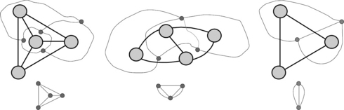
in which de is Euclidean distance. Points pi and pk are called Voronoi-adjacent iff pi ≠ pk and V(pi) ∩ V(pk) is a nontrivial straight line segment; the segment may be finite or infinite, but it must consist of more than one point. Figure 4.3 (right) shows Voronoi adjacencies between 10 grid points. Voronoi adjacencies in R2 will be discussed further in Chapter 13.

FIGURE 4.3 Left: 4-adjacencies between regions of a picture. Right: Voronoi adjacencies between selected grid points.
Polygonal tilings of the plane and partitions of 3D space into polyhedra also define adjacency graphs. Such a partition is called regular iff the intersection of two nondisjoint tiles or polyhedra is either a vertex, an edge, or a face.
Figure 4.3 (left) shows 4-adjacency between nine regions in a picture. An adjacency between two pixels p and q in a picture P is called valid iff p and q are P-equivalent (i.e., P(p)= P(q)); otherwise it is called invalid. The valid adjacencies do not define an adjacency graph, because P is not generally connected with respect to these adjacencies.
4.1.4 Types of nodes; region adjacencies
Nodes in a subset of an adjacency graph are classified as follows:
Definition 4.4
p ∈ M ⊆ S is called an inner node iff A(p) ⊆ M; otherwise it is called a border node.3 The set of inner nodes of M is called the inner set![]() of M, and the set of border nodes of M is called the border δM of M. A border node of S/M is sometimes called a coborder node of M.
of M, and the set of border nodes of M is called the border δM of M. A border node of S/M is sometimes called a coborder node of M.
3In graph theory [1073], it is called a node of attachment of M in S.
Evidently, ![]() and δM are disjoint. These concepts resemble the topologic concepts of the interior and frontier of a subset of a topologic space (see Section 3.1.7 and further discussion in Chapter 6). In a topologic space, a closed subset contains its frontier, but a proper open subset does not. A proper subset M of an adjacency graph has a nonempty border, but it may have an empty inner set. Class 5 in Figure 2.17 has five 1-components; only the 1-component M on the left has a nonempty inner set
and δM are disjoint. These concepts resemble the topologic concepts of the interior and frontier of a subset of a topologic space (see Section 3.1.7 and further discussion in Chapter 6). In a topologic space, a closed subset contains its frontier, but a proper open subset does not. A proper subset M of an adjacency graph has a nonempty border, but it may have an empty inner set. Class 5 in Figure 2.17 has five 1-components; only the 1-component M on the left has a nonempty inner set ![]() , which consists of two nodes.
, which consists of two nodes.
If the adjacency relation is one of the Aαs defined in Section 2.1, we use the terms α-region, α-inner set, or α-border or the symbols ![]() and δαM with α ∈{0,1,2,4,8,…}.
and δαM with α ∈{0,1,2,4,8,…}.
The connectedness relation ΓM partitions ![]() and δM into components called inner and border components of M.A component M such that
and δM into components called inner and border components of M.A component M such that ![]() consists of one border component. Figures 4.4 and 4.5 show the 1-border and 1-inner components of the set M defined by the union of the classes 2,3, and 5 shown in Figure 2.17. Note that, in these figures, we assume a finite rectangular grid; for an extended (infinite) grid, we would have a few more 1-border components.
consists of one border component. Figures 4.4 and 4.5 show the 1-border and 1-inner components of the set M defined by the union of the classes 2,3, and 5 shown in Figure 2.17. Note that, in these figures, we assume a finite rectangular grid; for an extended (infinite) grid, we would have a few more 1-border components.


In an adjacency graph S, the operation E of erosion (see Section 1.2.12 and Chapter 15) transforms M ⊆ S into ![]() , and the operation D of dilation transforms M into M ∪ A(M) (see below). For any L,M ⊆ S, we have the following:
, and the operation D of dilation transforms M into M ∪ A(M) (see below). For any L,M ⊆ S, we have the following:
In addition, D(M ⊆ L)= DM ⊆ DL. For any M ⊆ S, we have the following:
In this case, DE means that we first apply E and then D. O = DE is called opening, and C = ED is called closing. Figures 4.6 and 4.7 show examples of DM and CM = EDM based on 1-adjacency of 2-cells. Figure 4.8 shows an example of DM, D2M, and D3M based on 2-adjacency of 3-cells; here M contains only one 3-cell.

FIGURE 4.6 1-dilation of class 1 shown in Figure 2.17.

FIGURE 4.7 1-closing of class 1 shown in Figure 2.17.

FIGURE 4.8 Repeated 2-dilation starting with one 3-cell: balls of 3-cells of radii 0,1, 2, and 3 with respect to metric ∂2.
The set A(M) of all nodes adjacent to M ⊆ S (i.e., the set of all ![]() such that A(p) ∩ M = ø) is called the adjacency set of M. Evidently, if M is finite, so is A(M), and A(S)= A(ø) = ø. A(M) is the set of border nodes of
such that A(p) ∩ M = ø) is called the adjacency set of M. Evidently, if M is finite, so is A(M), and A(S)= A(ø) = ø. A(M) is the set of border nodes of ![]() ; this set is sometimes called the coborder of M. The number of complementary components of M is at most equal to the number of components of A(M), because every complementary component of M intersects A(M), and every component of A(M) is included in a unique complementary component.
; this set is sometimes called the coborder of M. The number of complementary components of M is at most equal to the number of components of A(M), because every complementary component of M intersects A(M), and every component of A(M) is included in a unique complementary component.
For any ![]() , there is at least one q ∈ δM such that p and q are connected with respect to M. If A(M) consists of only one component, the same is true for
, there is at least one q ∈ δM such that p and q are connected with respect to M. If A(M) consists of only one component, the same is true for ![]() . We also have
. We also have ![]() .
.
Because A is symmetric, we have A(M1) ∩ M2 ≠ 0 iff A(M2) ∩ M1 ≠ø so that A is symmetric. Because M1 and M2 are disjoint, A is irreflexive, so it is an adjacency relation on any partition of S.
Let R be a partition of S into regions and (possibly) the infinite background component. The undirected graph [R, A] is an adjacency graph; it is called the region adjacency graph of R. Figure 4.9 shows an example of a region adjacency graph defined by 1-adjacency of 2-cells. Figure 4.10 (left) shows the region adjacency graph for the picture in Figure 4.3 (left), and Figure 4.10 (right) shows the region adjacency graph for the picture in Figure 2.23, where node A represents the infinite background component. Region adjacency graphs will be discussed further in Chapter 7; see also Theorem 4.2

FIGURE 4.9 The region adjacency graph for the 1-regions shown in Figure 2.17.

FIGURE 4.10 Two region adjacency graphs. Left: for the picture on the left in Figure 4.3. Right: for the picture in Figure 2.23.
4.2 Some Basics of Graph Theory
Before continuing our discussion of adjacency graphs, we review some basic graph-theoretic concepts that are (potentially) relevant to digital geometry. In this section, G =[S, A] is a graph.
4.2.1 Nodes, paths, and distances
Let α0 = card(S) and α1 = card(A). G is finite iff ![]() . For any finite graph, we have the following:
. For any finite graph, we have the following:

The degree v(p) of node p is the number of edges that are incident with p; thus v(p) = card A(p). For example, all nodes in the infinite graph on the left in Figure 4.1 have degree 2 except for one, which has degree 4. For any finite graph, we have the following:
Nodes in a digraph have an in-degree and an out-degree, which are defined by the numbers of edges for which the node is initial or terminal. The maximum and sum of the in-degree and out-degree define a lower and an upper bound (respectively) for the degree of the node in the underlying undirected graph.
A path ρ is a sequence (p0, p1,…, pn) of nodes of G in which consecutive nodes are adjacent. The length λ(ρ) of ρ is the number n of consecutive pairs of nodes (i.e., the number of edges in the sequence).
A single node is a path ρ = (p) of length zero. A circuit is a path that begins and ends at the same node (i.e., pn = p0) and in which no edge occurs twice. A circuit of length n will be denoted with (p1,p2,…, pn). A loop in a pseudograph will be regarded as a circuit of length 1. There can be a circuit of length 2 in a multigraph but not in a simple graph. A proper subpath of a circuit is called an arc. A single node of a circuit is an arc of length 0. Two nodes p and q of G are called connected if there is a path (p0,…, pn) such that p0 = p and qn = q. G is called connected iff any two of its nodes are connected. Maximal connected sets of nodes of G are called components of G.
The distance dG (p, q) between two connected nodes p and q of G is the length of a shortest path connecting p and q. (If p and q are not connected, the distance between them is said to be infinite.) If G is connected, this distance is a metric, which is called the graph metric. Evidently, dG (p, q) = 0 iff q = p, and dG (p, q) = 1 iff pAq. Hence A(p) = {q ∈ S : dG(p,q) = 1} and N(p) = {q ∈ S : dG(p, q) ≤ 1}. Note that, if G is not connected, dG is a generalized metric in the sense that the axioms of a metric are satisfied (except that a distance value can also be infinite).
A shortest path connecting two nodes of G is sometimes called a geodesic. It can be found by simple breadth-first search [743]. Figure 2.4 illustrates two geodesics: in [Z2,A4] on the left and in [Z2,A8] on the right.
In a weighted graph G =[S, A, w], a positive real weight w(p, q) > 0 is assigned to every edge {p,q}∈ A. Note that w(p,q) = w(q,p). If p and q are not adjacent, we define w(p, q) to be infinite. A graph can be regarded as a weighted graph in which w(p, q) = 1 for all edges {p, q} ∈ A.
If we identify the nodes of a graph with points in Euclidean space, we can assign to each edge {p, q} a weight equal to the Euclidean distance between p and q. For example, in [Z2,A8], we have ![]() if p and q are 8-adjacent but not 4-adjacent, and w(p,q) = 1 if they are 4-adjacent. In a 3D picture with nonuniform spacing between voxels (e.g., different spacing between slices and within a slice), these spacings can be used to define weights.
if p and q are 8-adjacent but not 4-adjacent, and w(p,q) = 1 if they are 4-adjacent. In a 3D picture with nonuniform spacing between voxels (e.g., different spacing between slices and within a slice), these spacings can be used to define weights.
The total weight of a path in a weighted graph is the sum of the weights of all the edges on the path. A path between two nodes that has minimum total weight is called a shortest path.
The Shortest Path Problem is as follows: Given a connected weighted graph G =[S, A, w] and a node p0∈ S, find a shortest path from p0 to each q ∈ S. This is a special case of the distance field problem (see Section 3.1.8) in which we use minimum distances to a set of nodes instead of distance to the single node p0.
Dijkstra’s algorithm [268] (see Algorithm 4.2) solves the shortest path problem with a computational complexity of ![]() . This can be transformed into
. This can be transformed into ![]() if a heap data structure is used for the set {q ∈ S/Vi: D(q) <∞} of remaining nodes. Using the labels assigned in Step 2, we can construct a shortest path from any node q ∈ S back to p0. These labels also give the remaining shortest path lengths.
if a heap data structure is used for the set {q ∈ S/Vi: D(q) <∞} of remaining nodes. Using the labels assigned in Step 2, we can construct a shortest path from any node q ∈ S back to p0. These labels also give the remaining shortest path lengths.
Figure 4.11 shows an application of Dijkstra’s algorithm to a simply 4-connected region (shown in the grid cell model; for an informal definition of “simply connected,” see Section 1.2.6). We choose a start node p on the border of the component and find all shortest 4-paths from p to nodes in the component with

FIGURE 4.11 A start node p; nodes (shaded) with distances to p that are local maxima; and a shortest path to the shaded node farthest from p.

lengths that are local maxima; this maps the component into a set of 4-arcs. The figure shows a shortest path to a node farthest from p. (“Thinning ” algorithms that map components into sets of 4-arcs are discussed in Section 16.3.)
The eccentricity e(p) of a node p of a finite connected graph G = [S, A] is the greatest distance max{dG(p, q): q ∈ S} from p to any node of S. Dijkstra’s algorithm can be used to calculate e(p). The radius r(G) and the diameter d(G) are (respectively) the minimum and maximum eccentricities of all of the nodes of S. Thus p is called a central node of G iff e(p)= r(G); the set of central nodes is called the center of G. Figure 4.12 shows the centers of some 4-connected sets of grid points in the graph defined by A4.
An Eulerian path in G is a path that contains all of the edges of G; see the historic comments at the beginning of Section 1.2.5. A graph is called Eulerian iff it has an Eulerian circuit.
A connected graph G is Eulerian iff every node of G has even degree, and G has an Eulerian path iff it has at most two nodes of odd degree (see Figure 4.13); in the latter case, the path starts at one of the nodes that has odd degree and ends at the other. (Note that there cannot be exactly one node of odd degree.) It follows that the existence of Eulerian paths or circuits can be determined, and Eulerian paths can be found in computation time-linear in the number of nodes.

A path that visits each node of G exactly once is called Hamiltonian. (In 1857, the London toymaker J. Jaques manufactured a puzzle called the “icosian game ” that involved finding such a path along the edges of a dodecahedron. The toymaker paid 25 pounds to Sir W.R. Hamilton for the rights to the puzzle. Hamilton proudly told Jaques that his bankers considered him at this point to be a man of business, because he had obtained cash for one of his inventions [408].) A graph that has a Hamiltonian circuit is called a Hamiltonian graph. Figure 4.14 shows examples of Hamiltonian graphs; they are planar representations (see Figure 4.17) of the vertices, edges, and faces of the five Platonic solids: convex polyhedra with faces that are congruent convex regular polygons. There are exactly five such solids (Euclid): the tetrahedron, the octahedron, the cube, the icosahedron, and the dodecahedron, which have 4, 6, 8, 12, and 20 vertices, respectively. The 4-adjacency grid Gm,n is a Hamiltonian graph if either m or n is even; to obtain a Hamiltonian circuit, start at the lower left corner, go all the way to the right, then zigzag up (“on the right ”) and down (“on the left ”) until the start node is reached again. Note that, for m,n ≥ 4, such a Hamiltonian circuit is not uniquely defined.

FIGURE 4.14 Five examples of Hamiltonian graphs: planar graphs representing the five Platonic solids.
The problem of finding a Hamiltonian circuit in a graph or deciding whether one exists is NP-complete.4 A connected graph G with n ≥ 3 nodes has a Hamiltonian circuit if v(p) + v(q) ≥ n for every pair of nonadjacent nodes p and q of G [272].
4.2.2 Special types of nodes, edges, and graphs
A node of degree 0 is called isolated and is a component of G. A node of degree 1 is called an end node. The edge incident with an end node is called a pendant edge.
A cut node is a node such that, if it is removed from S along with all of the edges incident with it, the number of components of G increases. For example, the graph in the middle in Figure 4.1 has two cut nodes.
If G is connected, its node connectivity is the smallest number of nodes for which removal from S disconnects G or completely deletes it. G is called k-strong iff its node connectivity is at least k. If G is connected, it is at least 1-strong; if G has no cut nodes, it is at least 2-strong.
A bridge is an edge of G for which removal from A disconnects G. An edge of a connected graph is a bridge iff it does not belong to any circuit.
A finite graph that has no circuits is called a forest, and, if it is also connected, a tree. Any tree that has more than one node has at least one pendant edge.
A proof will be given in Section 7.3.2.
A rooted tree is a tree with a distinguished node called the root. We recall (Section 4.2.2) that a region adjacency graph has at most one node that represents an infinite component. If the graph is a tree, it is usual to choose this node as the root of the tree. Figure 4.15 shows the region adjacency trees defined by the (4,8)- and (8,4)-adjacency structures of a binary picture P in which the pixels of ![]() are represented by filled dots.
are represented by filled dots.

FIGURE 4.15 (4,8)- (on the left) and (8,4)- (on the right) adjacency structures defined by the set ![]() of 1s of a binary picture. Below: The rooted region adjacency trees for the regions and complementary regions of
of 1s of a binary picture. Below: The rooted region adjacency trees for the regions and complementary regions of ![]() .
.
The distances of the nodes from the root of a rooted tree define layers or levels in the tree. Layer −1 is the empty set, and Layer 0 contains only the root. For n ≥ 0, Layer n + 1 contains all nodes that are not in Layer n −1 but that are adjacent to a node in Layer n. Nonroot nodes of a rooted tree that have degree 1 are called leaves.
A spanning tree of a graph G =[S, A] is a subgraph of G that is a tree and that has vertex set S. A minimum-length spanning tree is a spanning tree with the fewest possible edges. For example, the minimum-length spanning tree of a 4-adjacency grid Gm,n is defined in terms of the Manhattan distance d4. Starting the construction of a minimum-length spanning tree at the center of a graph minimizes the diameter of the tree [997].
G =[S,A] is called bipartite iff S can be partitioned into two disjoint subsets S1 and S2 such that each edge in A joins a node in S1 to a node in S2. For example, one component of the graph on the right in Figure 4.1 is bipartite. The 4-adjacency grid Gm,n is bipartite; the nodes can be partitioned like the squares on a chessboard.
Gm,n is even complete bipartite (i.e., there exists a partition of its node set into two subsets S1 and S2 such that every node in S1 is adjacent to every node in S2). If S1 has n nodes and S2 has m nodes, the complete bipartite graph is denoted by Kn,m. One component of the graph on the right in Figure 4.1 is K3,3. This graph arises in the puzzle of “three houses, each connected to the electricity, water, and gas companies.”
A graph is called complete if every pair of its nodes is adjacent. For a finite complete graph, we have ![]() . The complete graph that has α0 = n nodes is denoted by Kn. Evidently, Kn is n-strong. K1 consists of one isolated node, K2 consists of one pair of adjacent nodes, and K3 consists of a circuit of length 3 (a triangle).
. The complete graph that has α0 = n nodes is denoted by Kn. Evidently, Kn is n-strong. K1 consists of one isolated node, K2 consists of one pair of adjacent nodes, and K3 consists of a circuit of length 3 (a triangle).
Renaming the nodes in a graph leads to an isomorphic graph. Formally, two graphs [S1,A1] and [S2,A2] are isomorphic iff there is a one-to-one mapping f from S1 onto S2 such that each edge {p, q} in A1 maps onto an edge {f (p),f(q)} in A2 and this mapping of A1 onto A2 is one-to-one. We can now say more precisely that one of the components of the graph on the right in Figure 4.1 is isomorphic to K3,3. Figure 4.16 illustrates graphs that are isomorphic to K3,3 and K5. The computational problem of determining whether or not two finite graphs are isomorphic is NP-complete.


FIGURE 4.17 The planar graph (below) represents all the faces, edges and vertices of the convex polyhedron (above).
The nodes of a graph have no coordinates; there is no specific way to draw a graph, for example, in the plane. A graph is called planar iff it allows a planar drawing5 (i.e., it can be drawn in a plane in such a way that its edges are drawn as simple arcs that intersect only at nodes). For example, K1, K2, K3, and K4 are planar, but K5 is not; the adjacency structure [Z2,A4] is planar, but [Z2,A8] is not. There are algorithms with linear run times (in the number of nodes) for deciding whether or not a given finite graph is planar; the first such algorithm was published in [443], and it is an iterative version of a method proposed in [53] and correctly formulated in [367]. The crossing number of a graph is the smallest possible number of intersections of edges (other than at nodes) for any drawing of the graph in a plane. A graph with crossing number 0 is planar. Determining the crossing number of a graph is an NP-complete problem.
With any polyhedron Π, one can associate a graph G as follows: the vertices of Π are represented by the nodes of G, and two nodes of G are joined by an edge iff the corresponding vertices of Π are joined by an edge of Π. The following theorem was proved by E. Steinitz (1871–1928):
Figure 4.17 shows a graph associated with a convex polyhedron.
A planar drawing of a finite planar graph partitions the plane into faces. The frontier of each face defines a cycle of consecutive arcs that join pairs of points p and q where {p, q} is an edge in the graph; this cycle corresponds to a circuit in the graph. Let α2 be the number of faces in such a drawing. Using Euler’s formula,6
we know that α2 is uniquely defined for any finite planar graph (i.e., it depends on the graph but not on the drawing). For example, for K1 and K2, we have α2 = 1, and, for K3, we have α2 = 2.
A planar drawing of a finite planar graph has α2− 1 bounded faces (its internal faces) and one infinite face (its external face). (Formula 4.5 also counts the external face; otherwise, 2 needs to be replaced with 1. The formula is also correct for drawing a planar graph on a sphere, which results in bounded faces only.) For example, any planar drawing of K3 has one internal and one external face. For any finite planar graph, we have the following:
where the sum is taken over all of the cycles ρ defined by all of the faces of a planar representation of the graph. (We recall that λ (ρ) is the length of ρ.)
The merging of two adjacent nodes p and q in a graph [S, A] is defined by replacing p and q with a new node r that is adjacent to every node in S/{p, q} to which p or q was originally adjacent. A finite sequence of merging operations is called a contraction.
Efficient planarity testing algorithms are not based on this theorem.
The chromatic number of a (finite) graph is the smallest number of colors needed to color the nodes of the graph so that adjacent nodes have different colors. For example, any bipartite graph has chromatic number 2, and the complete graph Kn has chromatic number n −1. The problem of calculating the chromatic number of a finite graph is NP-complete.
A geographic map (see Figure 4.2) can be represented by a finite planar graph in which each country is represented by a node, and there is an edge between two nodes iff the intersection of the frontiers of any two countries consists of more than a set of isolated points. (The intersection may consist of several disjoint arcs.) Any planar drawing of a finite planar graph is a planar drawing of such a “map graph.”
This theorem has a long and interesting history of published “proofs ” that were later found to be incorrect [89,410]. The problem was first stated in 1852, and many mathematicians contributed to its eventual solution [25].
Given a planar drawing of a (finite or infinite) planar graph, the geometric dual of the drawing is constructed by choosing a point in each face of the drawing (including the external face), and, if the frontiers of two faces have a simple arc γ in common, joining those faces ’ points with a simple arc that crosses γ. The result of this construction is a planar drawing of a multigraph. Figure 4.18 shows three examples. The planar drawing on the left is self-dual, because the drawing and its geometric dual are isomorphic. The planar drawing of [Z2, A4] is also self-dual. The other two planar drawings in Figure 4.18 have duals that are multigraphs but not graphs. (Note that multigraphs occur only if the original planar graph is not connected or because of the external face.) Thus the dual of a planar drawing of a finite planar graph is more general than a planar graph representation of a geographic map, where we excluded multiple edges.
4.3 Oriented Adjacency Graphs
There are infinitely many ways to draw a finite planar graph. We call two drawings equivalent iff the clockwise order of the edges around each node is the same in both drawings. This defines equivalence classes of planar drawings, which are called combinatorial embeddings.
4.3.1 Local circular orders
In this section, we introduce the concept of a “local ” circular order of the edges incident with a node of a graph and generalize it so that it can be applied to any (not necessarily finite or planar) adjacency graph.
The directional code shown in Figure 2.31 specifies a local circular order on the grid points of [Z2,A8] (i.e., a cyclic ordering of the grid points that are 8-adjacent to any given grid point). Such orders provide a basis for defining border tracing routines.
Let [S, A] be an adjacency graph. In a local circular order ξ(p) at node p ∈ S, the nodes {q1, qn) of A(p) appear exactly once each. We can use these local orders to trace (directed) edges in [S, A] as follows: if we arrive at p from qi∈ A(p), we move next to qk, where k = i + 1 (modulo n).
Figure 4.19 shows all possible ways of defining a local circular order on [Z2,A4]. For example, in case (A), for any grid point p = (x,y)∈ Z2, we have ξ(p) = <, (x,y + 1), (x + 1, y), (x,y – 1)). Let us denote the directions from (x,y) to these four neighbors with 1, 2, 3, and 4 (modulo 4). If we arrive at p from below (direction 4), we proceed (modulo 4) in direction 1 to a new grid point. At the new grid point, we arrive from direction 3 and proceed in direction 4. At the next grid point, we arrive from direction 2 and proceed in direction 3, and, at the next grid point, we arrive from direction 1 and proceed in direction 2; this closes a circuit of length 4 in [Z2, A4]. Note that, in this example, we used the same local circular (A) at every node; we will do this from now on.

Any move from a grid point p to one of its neighbors q initiates a (directed) path defined by the local circular order. Figure 4.20 shows all possible initiated paths using each of the local circular orders shown in Figure 4.19. The initiated paths are infinite in cases (B) to (E); only cases (A) and (F) lead to finite paths (circuits), which are always of length 4. We call these finite paths cycles.
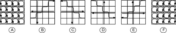
Local circular orders (A) and (F) generalize the cycles used to trace borders in planar drawings, where we use either the clockwise or counterclockwise order of the edges incident with each node.
An oriented adjacency graph [S,A,ξ] is defined by an adjacency graph [S,A] (having properties A1 through A3; see Section 4.1.3) and an orientation ξ, defined by local circular orders of the adjacency sets, which satisfies the following:
Any finite adjacency graph obviously has this property (i.e., any finite [S, A] and any ξ define an oriented adjacency graph).
For [Z, A4], circuits of length 4 are the only possible cycles, and only the orientations (A) and (F) of Figure 4.19 lead to oriented adjacency graphs. For any [Gm,n,A4], in cases (A) and (F), we obtain cycles of length 4 plus one additional cycle, which we say circumscribes Gm,n (and “defines ” an external face).
4.3.2 The Euler characteristic and planarity
Let α2 be the number of cycles of a finite oriented adjacency graph [S, A, ξ]. (Note that a cycle cannot be decomposed into two or more cycles.) If [S, A] is planar, it has α2 faces.
We recall that α0 = card (S),α1 = card(A)/2, and v(p) = card(A(p)). Equation 4.4 is true for any finite graph; hence, for any finite oriented adjacency graph, the following is given:
Equation 4.6 also generalizes to arbitrary finite oriented adjacency graphs,
where λ(ρ) is the length of cycle ρ and the sum is taken over all cycles in [S, A, ξ].
From property A2, it follows that there are at least α0 −1 edges (i.e.,α1 ≥α0 −1). Two nodes can be connected by at most one undirected edge so that α1 ≤α0(α0 – 1)/2. A single node (α0 = 1 and α1 = 0) defines a degenerate cycle (α2 = 1). A given (nonplanar) finite adjacency graph [S, A] can have different numbers α2 of cycles depending on its orientation ξ.
The Euler characteristic X, which is also known as the Euler number, will be characterized in Section 6.4.5 as a topologic invariant for finite Euclidean complexes that consist of bounded sets. From Equation 4.5 (Euler ’s formula), we know that χ = 2 for the surface of a simple polyhedron so that χ = 1 (not counting the unbounded external face) for the finite planar graph that represents the surface of the polyhedron. In terms of the concepts in Chapter 6, a graph defines a finite one-dimensional complex of nodes and arcs. A planar graph defines a finite number of bounded internal faces and one unbounded external face. (If we project the planar graph onto a sphere, the external face becomes a bounded face.) In this section, we deal with graphs that are not necessarily planar. To simplify the notation, we regard all of the cycles of an oriented adjacency graph as “faces,” including unbounded external faces, and indicate this with the superscript +.
The Euler characteristic of a finite oriented adjacency graph [S, A, ξ] is defined to be χ = α0 −α1 + (α2 − 1). Let χ + = χ + 1 = α0 –α1 +α2. Then we have the following:
Theorem 4.6
χ+≤ 2 for any finite oriented adjacency graph.
Proof The proof is by induction based on repeated addition of new edges to a finite oriented adjacency graph. If α0 = 1,α1 = 0, and α2 = 1, we have χ+ = α0−α1 +α2 = 2. Suppose χ+ ≤ 2 for G =[S,A,ξ]. We can add an edge to G, thereby producing a graph Gnew in two ways:
1. Add a new node q to S, and connect q with a new edge to an existing node p of S.
2. Add a new edge to A by connecting two nodes p and q of S that were not connected by an edge in A.
In the first case, we increase both α0 and α1 by 1. The local circular order ![]() becomes
becomes ![]() . (pi, p) initiated a cycle
. (pi, p) initiated a cycle ![]() in G and initiates a cycle
in G and initiates a cycle ![]() in Gnew. All other cycles in G remain unchanged. Thus α2 does not change, so we have the following:
in Gnew. All other cycles in G remain unchanged. Thus α2 does not change, so we have the following:
In the second case, suppose first that some cycle of G contains both p and q. This cycle ![]() splits into two cycles,
splits into two cycles, ![]() and
and ![]() , so that the following is true:
, so that the following is true:
Finally, suppose p and q are in two different cycles of G, for example,![]() and
and ![]() . The new edge links these two cycles, thereby resulting in the cycle
. The new edge links these two cycles, thereby resulting in the cycle ![]() , so that the following is given:
, so that the following is given:
This proof also implies that the Euler characteristic χ + 1 of a finite oriented adjacency graph is always a multiple of 2 (…, 2,0,−2,−4,…).
Theorem 4.6 suggests the following generalization (and formalization) of the concept of planarity, which was defined in Section 4.2.2 in a more informal way:
This definition is consistent with graph theory and combinatorial topology:χ = 1 for any planar drawing of a planar graph, and each such drawing defines an orientation for the graph.
If local circular orders are defined for all of the adjacency sets of K3,3 or K5,it can be verified that the resulting finite oriented graph always has χ+ < 2. It follows that any finite undirected graph that has a subgraph that can be contracted into either K3,3 or K5 has χ+ < 2 for any orientation defined on it. By Kuratowski’s theorem, it follows that a finite connected graph is planar iff it has at least one orientation for which χ+ = 2.
The infinite 4-adjacency grid [Z2,A4], using either the clockwise (A) or counterclockwise (F) local circular order (see Figure 4.19), is planar. Any connected subset of [Z2, A4] is also planar; thus the Euler characteristic remains χ+ = 2 for any connected region of a grid under 4-adjacency. An infinite switch-adjacency grid [Z2, As] (see Section 2.1.3) is also planar, and its connected regions too are planar.
The infinite 8-adjacency grid [Z2,A8] (e.g., with counterclockwise local circular orders) is nonplanar. In fact, let Gm,n(m,n ≥ 2) be a rectangular oriented subgraph of [Z2,A8]. Then (see Figure 4.21)χ + = −2(m − 2) for m ≥ 2 and n = 2(α0 = 2m,α1 = 5m − 4, and α2 = m); and χ + = −2(3m − 4) for m ≥ 2 and n = 4(α0 = 4m,α1 = 13m−10, and α2 = 3m−2). For example, for m = 6 and n = 4, we have χ + = −28. In a picture defined on an 8-adjacency grid, the Euler characteristic of a connected region (its “degree of planarity ”) decreases with the size of the region.

FIGURE 4.21 Unlimited decrease of the Euler characteristic χ + in the infinite 8-adjacency grid. The numbers below the rectangular oriented graphs are values of χ+.
The planar graphs representing the Platonic solids (see Figure 4.14) are examples of finite regular planar adjacency graphs. Of course, their sets of nodes are far too small to serve as 2D grids for digital pictures. For infinite sets of nodes, there are only three regular planar adjacency graphs: the orthogonal grid on Z2 with λ(g) = v(p) = 4, the triangular grid with λ(g) = 3 and v(p)= 6, and the hexagonal grid with λ(g) = 6 and v(p) = 3. We also have their isomorphic structures such as the dual of the 4-adjacency grid in the grid cell model with nodes in ![]() .
.
Rectangular subsets of planar or nonplanar infinite regular adjacency graphs are “popular ” 2D grids for digital pictures. However, note that nonplanarity allows a finite simply 8-connected set to have (any of) infinitely many Euler characteristics, as illustrated in Figure 4.21.
4.3.3 Atomic and border cycles
A subset M ⊆ S induces a substructure [M, AM, ξM] of an oriented adjacency graph [S, A, ξ] where AM contains only those adjacency pairs {p, q} such that p,q ∈ M and {p, q} ∈ A, and where, for any p ∈ M,ξM (p) is the reduced local circular order defined by deleting from ξ(p) all nodes that are not in M. Such a substructure is an oriented adjacency graph iff M is connected with respect to AM.
Let ![]() be the number of nodes,
be the number of nodes, ![]() the number of edges or adjacency pairs, and
the number of edges or adjacency pairs, and ![]() the number of cycles in [M,AM, ξM]. Then the Euler characteristic
the number of cycles in [M,AM, ξM]. Then the Euler characteristic ![]() of
of ![]() is at least equal to the Euler characteristic χ of [S, A, ξ]. On the other hand, we have the following, where
is at least equal to the Euler characteristic χ of [S, A, ξ]. On the other hand, we have the following, where ![]() is the number of components of M in [S, A]:
is the number of components of M in [S, A]:
The cycles of [M, AM,ξM] may differ from the cycles of [S, A, ξ]. Let (p, q) be a directed edge in [M,AM,ξM], let ρ1 be the cycle generated by (p,q) in [M,AM,ξM], and let ρ2 be the cycle generated by (p, q) in [S, A, ξ].
For example, there are five border cycles in Figure 4.22, with α0 = 37,α1 = 46, and α2 = 11 for the component on the left;α0 = 4,α1 = 3, and α2 = 1 for the component in the middle; and α0 = 28,α1 = 28, and α2 = 2 for the component on the right.

For any M ⊂ S, [M,AM, ξM] has at least one border cycle. Each border cycle of [M,AM, ξM] contains at least one border node of M, and each border node is incident with at least one border cycle.
4.3.4 The separation theorem
Let (r, q) be a directed edge in [S,A], M ⊆ S, q ∈ δM, and r ∈ (SM). We call (r,q), a directed invalid edge from ![]() to M. An undirected edge between
to M. An undirected edge between ![]() and M is invalid iff one of its two directions is invalid.
and M is invalid iff one of its two directions is invalid.
A directed invalid edge (r,q) points to a cycle in [M,AM, ξM] if (q,p) is the directed edge such that p is the first node of M that follows r in the (original) local circular order ξ(q). Figure 4.23 shows an example; for the directed invalid edges (r,q), (s,q), and (t,q), p is the next (and in ![]() , the only) node in M, and
, the only) node in M, and ![]() initiates the border cycle. Every directed invalid edge points to exactly one border cycle in [M,AM, ξM]. This defines a partition of all (directed or undirected) invalid edges into equivalence classes; each class is the set of all (directed or undirected) invalid edges that are assigned to a given border cycle.
initiates the border cycle. Every directed invalid edge points to exactly one border cycle in [M,AM, ξM]. This defines a partition of all (directed or undirected) invalid edges into equivalence classes; each class is the set of all (directed or undirected) invalid edges that are assigned to a given border cycle.

FIGURE 4.23 The directed invalid edges (r, q), (s, q), and (t, q) all point to the border cycle initiated by (q,p) in the substructure defined by the filled dots.
This separation theorem can be compared with the Jordan-Veblen curve theorem (see Chapter 7) in the Euclidean plane. Let M be connected, let (r, q) be a directed invalid edge from ![]() to M, and let
to M, and let ![]() be the border cycle in [S,A,ξ] to which (r,q) points. Then, for any p ∈ M and any path ρ =(p,…, r), we have G(p) ∩ {q1…, qn} ≠ø where G(p) is the set of all nodes of p. In other words, a border cycle establishes separations in a planar oriented adjacency graph based on “tracing ” border cycles.
be the border cycle in [S,A,ξ] to which (r,q) points. Then, for any p ∈ M and any path ρ =(p,…, r), we have G(p) ∩ {q1…, qn} ≠ø where G(p) is the set of all nodes of p. In other words, a border cycle establishes separations in a planar oriented adjacency graph based on “tracing ” border cycles.
Let [S, A, ξ] be an oriented adjacency graph (not necessarily planar), and let M ⊂ S be a finite proper subset of S. We consider the computational problem of finding (“tracing ”) all border cycles of M.
Note first that the border cycles of different components of M are disjoint, so we can consider each component of M independently. To determine the components of M we can use the recursive FILL procedure in Algorithm 4.1. We choose a node p in M and find (“fill ” or “label ”) all of the nodes connected to p; this provides the first component of M. As long as unlabeled nodes still remain in M, we repeat this procedure to obtain all of the components of M, one for each repetition of the procedure.
Every directed invalid edge points to exactly one border cycle. For each component A of M, we generate a list L of all directed invalid edges. We choose any of these edges and trace the border cycle to which it points (see the following discussion). During tracing, we delete all of the assigned directed invalid edges from L. If there is still an undeleted directed invalid edge on L, we repeat the process; this generates all of the border cycles of A. L can be generated in a scan through A if all of the detected border nodes p ∈ δA form directed invalid edges (q,p) with all nodes ![]() ; these edges will be inserted into L.
; these edges will be inserted into L.
ALGORITHM 4.3 The border tracing algorithm [1111].
1. Let (q0, p0):=(q,p),i := 0, and k := 0.
2. Let ![]() be the local circular order at pi. If
be the local circular order at pi. If ![]() , go to Step 4.
, go to Step 4.
3. Node q is another node on the border cycle. Let i := i + 1 and pi : = q. Let ![]() be the local circular order at pi. If q ∈ A, go to Step 3; otherwise, let k := i −1, and go to Step 4.
be the local circular order at pi. If q ∈ A, go to Step 3; otherwise, let k := i −1, and go to Step 4.
4. If (q,pi) = (q0, p0), go to Step 5. Otherwise, let k := k + 1 and qk : = q, and go to Step 2.
5. We are back at the original directed invalid edge (q,p). The border cycle is ![]() .
.
The algorithm for tracing the border cycle pointed to by a given directed invalid edge (q,p) is given in Algorithm 4.3 The algorithm terminates because of property A4. The deletion of all directed invalid edges may lead to a separation if [S, A, ξ] is nonplanar, but the border tracing procedure applies even to nonplanar graphs.
4.3.5 Holes
Let G =[S,A,ξ] be an infinite oriented adjacency graph, and let M be a finite connected subset of S. Using property A3 (see Section 4.1.3), M has exactly one infinite complementary component. Any finite complementary component of M is called a hole of M. If S = Zn and the hole is α-connected, we call it an α-hole. For example, finite connected subsets of [Z2,A4] can have 8-holes that consist of several 4-holes.
If G is planar, M has exactly one border cycle, called its outer border cycle, which separates M (see Theorem 4.7) from its infinite complementary component. All other border cycles of M are called inner border cycles. If complementary component A of M is separated from M by border cycle ρ of M, we say that A is assigned to ρ.
Figure 4.24 illustrates this definition. Two complementary 1-components belong to the background 1-component of class 1; two complementary 1-components are proper 1-holes (separated by a 1-component from the background 1-component); and two complementary 1-components are improper 1-holes (not separated by a 1-component from the background 1-component).

FIGURE 4.24 Three 1-components and six complementary 1-components (of class 1 in Figure 2.17). 1-holes in the grid cell model are 4-holes in the grid point model.
The cover c(M) of M is the union of M with all of its proper holes. c(M) has no inner border cycles, but it has an outer border cycle that may separate improper holes from c(M). Finite complementary components of a finite or infinite connected subset of an infinite planar oriented adjacency graph do not have proper or improper holes.
Planarity of the oriented adjacency graph is crucial for the definition of inner and outer border cycles. A border cycle circumscribes the proper or improper holes assigned to it. The set M in Figure 4.25 has 14 border cycles: 10 “triangles ” (small artifacts of atomic cycles); three border cycles that circumscribe one proper 4-hole and two improper 4-holes; and one border cycle ρ that circumscribes the union of M with its proper and improper 4-holes. ![]() has eight border cycles: six “triangular artifacts ”; one border cycle for the proper 4-hole in M; and one border cycle that “penetrates ”ρ (i.e.,ρ does not separate M from its background).
has eight border cycles: six “triangular artifacts ”; one border cycle for the proper 4-hole in M; and one border cycle that “penetrates ”ρ (i.e.,ρ does not separate M from its background).

4.3.6 Boundaries
The following definition applies to planar and nonplanar oriented adjacency graphs. In Figure 4.25 (left), all undirected invalid edges assigned to any border cycle of M have been removed.
This definition resembles the discussion in [202] about the “boundary between layers of white and black marbles.” (We use light gray in Figure 4.26 instead of black.) Such a boundary is neither a set of white nor of black marbles and is better described as the “space between the white and black layers ” (see the left of Figure 4.26) or as neighboring pairs of white and black marbles (see the right of Figure 4.26).

FIGURE 4.26 Example of layers of white and light-gray marbles as discussed in [202]. Left: the space between the layers is dark gray. Right: marbles that have neighboring marbles of the other color are dark gray.
When we use Gauss digitization (see Section 2.3.1), the boundary of G(S) (in the grid point model) consists of edges that cross the frontier of G(S); see Figure 4.27. Such a boundary can be represented by an ordered sequence of midpoints of those edges. Figure 4.28 shows examples of such polygonal representations of boundaries.

FIGURE 4.27 Left: the border (black vertices) and boundary (bold edges) of G(D) in the grid point model, where D is a disk. Right: the border and boundary of G(D) in the grid cell model.

FIGURE 4.28 Left: no problem occurs in the case of the disk. The other three pictures show midpoint sssuences that “prefer ” connections between background points or between object points and a doubly oriented midpoint sequence that treats background and object points equally.
The edges can be found by comparing every 2 × 2 block of pixels with a set of templates (see Figure 4.29), and, for each match, copying (generating) the “detected ” edge(s).
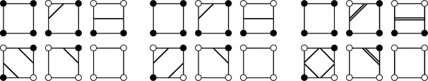
FIGURE 4.29 Left: look-up table with a preference for connections between background points. Middle: preference for connections between object points. Right: doubly oriented edges.
If we use the left or middle look-up table in Figure 4.29, the plane is segmented into polygons. The object polygons can be regarded as closed sets in the Euclidean topology, and the background polygons as open (or vice versa). This defines a partition of the plane into pairwise disjoint sets with frontiers that are the polygonal boundaries. We can assume that each doubly oriented edge shown on the right in Figure 4.29 is actually two directed edges with a small space between them. This leads to a segmentation of the plane into pairwise disjoint (even “nontouching ”) polygons. The space between the polygons is a representation of the boundary; this is similar to a situation where a wall is built out of stones and the boundary is the mortar between the stones.
4.3.7 Some combinatorial results
This section gives formulas for some topologic invariants (see Definition 6.9) of isothetic polygons using the more abstract language of infinite planar regular oriented adjacency graphs. We use the hexagonal and trigonal grids (see Definition 4.7) as well as the orthogonal grid.
We begin by recalling Equations 4.4 and 4.7. Let G =[S, A,ξ] be a finite oriented adjacency graph with α0 = card(S) and α1 = card(A)/2. Let the following
be the mean outdegree of a node and the mean length of a cycle where the second sum is over all cycles of G. Then the following is true,
which implies the following:
This equation also applies to infinite oriented adjacency graphs if both means are well defined, because 2/α1 goes to zero for infinite graphs.
A regular oriented adjacency graph Gv,λ represents a regular tiling (of some surface) and vice versa. For examples of finite regular tilings, see Section 7.6—Exercises 7 and 8 (for the surface of a sphere), 9 and 10 (for the plane), 11 (for the surface of a torus), and 12 (for a closed surface). For infinite graphs (e.g., on a plane), Equation 4.9 has only three integer-valued solutions: v = λ = 4; v = 3 and λ = 6; and v = 6 and λ = 3. We will assume that S = Z2 in these three infinite planar Gv,λs (see Exercise 10 in Section 7.6).
Consider a finite subgraph of one of these three Gv,λs defined by a finite subset M ⊆ Z2. We first consider the case in which M has only one border cycle, for example, of length l. Following Definition 6.13, we call such an M simply connected. Let k be the number of invalid undirected edges between ![]() and M; see Figure 4.30 for an example. Because Gv,λ is planar, Equations 4.4 and 4.7 give us the following:
and M; see Figure 4.30 for an example. Because Gv,λ is planar, Equations 4.4 and 4.7 give us the following:
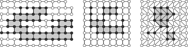
FIGURE 4.30 v = 3,λ = 6,α0 = 49,α1 = 59,α2 = 12, l = 52, k = 29, f = 11 (left); v = 4,λ = 4,α0 = 23,α1 = 30,α2 = 9, l = 28, k = 32, f = 8 (middle); and v = 6,λ = 3,α0 = 18,α1 = 32,α2 = 16, l = 19, k = 44, f = 15 (right).
so that the following is true:
If we regard v and λ as parameters of Gv,λ, the relationship between l and k is defined by the number α1 of undirected edges in the subgraph defined by M. For the Gv,λs we have 2v + 2λ − vλ = 0.
In other words, the relationship between the number of invalid edges and the length of the border cycle depends only on the parameters v and λ.
Now suppose M has r ≥ 1 border cycles. Instead of Equations 4.10, 4.11, and 4.12, we have the following:
In these, li is the length of border cycle i (1 ≤ i ≤ r) and ki is the number of invalid edges that connect ![]() with nodes on border cycle i. For the Gv,λs, we have 2v + 2λ − vλ = 0, so that the following is true:
with nodes on border cycle i. For the Gv,λs, we have 2v + 2λ − vλ = 0, so that the following is true:
The outer border cycle of M is the same as the outer border cycle of its cover c(M) (the union of M with all its proper holes), so Theorem 4.8 is valid for c(M). It follows that we always have vlr − λkr + vλ = 0 where r is the index of the outer border cycle of M. Subtracting this equation from Equation 4.17 gives the following:
The r − 1 inner border cycles of M can be regarded as independent events, and Equation 4.18 splits into r − 1 equations vli – λki + vλ = 0,1 ≤ i ≤ r −1.
This theorem provides a simple algorithm for deciding whether a traced border cycle (see Algorithm 4.3) is inner or outer by keeping track of k and l during border cycle tracing.
From Equation 4.17, it follows that r = 2 + L/λ − K/v. The total length L of all border cycles and the total number K of all invalid edges allow us to calculate the number r of border cycles, which is a topologic invariant of M. Note that L and K can be accumulated by examining all 4-neighborhoods of points in M; border cycle tracing is not necessary.
Let f be the number of atomic cycles of M. Combining Theorem 4.8 and Equations 4.10, 4.11, and 4.12 gives the following:
For any of the Gv,λs, we have 1/λ + 1/v = 1/2. This proves the following:
This theorem is a graph-theoretic generalization of a result proved by G. Pick (1899)7 for the regular orthogonal grid (v = λ = 4): the area f of a simple grid polygon (a simple polygon that has grid points as vertices) satisfies f = α0 − l/2 − 1, where α0 is the number of grid points in the polygon and l is the number of grid points on the frontier of the polygon. For example, for a grid square, we have α0 = l = 4 and f = 1.
Theorem 4.10 applies to outer border cycles. For an inner border cycle ρ, let α0 be the number of nodes of Gv,λ/M surrounded by ρ (“in the interior of ρ”), and let f be the number of atomic cycles of Gv,λ defined by these α0 nodes and the nodes of ρ. Then we have the following:
Note that an inner border cycle can separate several proper holes from M; Theorem 4.11 applies to the union of these holes.
Figure 4.31 shows examples; k is the number of invalid edges assigned to the inner border cycle, and we have shaded the atomic cycles of the proper holes assigned to the inner border cycle. On the left, we have three proper holes and one atomic cycle in one of them; in the middle, we have one proper hole and one atomic cycle; on the right, we have one proper hole and two atomic cycles. Let m be the total number of atomic cycles of all the proper holes assigned to the given inner border cycle. The remaining f – m atomic cycles, defined by nodes in the complementary set ![]() and on the inner border cycle, are boundary cycles, where the boundary specifies the “space between.” The λm edges of the boundary cycles include k invalid edges, the length l of the inner border cycle, and the sum of the lengths li of the outer border cycles of the n > 0 proper holes assigned to the inner border cycle:
and on the inner border cycle, are boundary cycles, where the boundary specifies the “space between.” The λm edges of the boundary cycles include k invalid edges, the length l of the inner border cycle, and the sum of the lengths li of the outer border cycles of the n > 0 proper holes assigned to the inner border cycle:
Together with Theorems 4.10 and 4.11, this implies the following:

FIGURE 4.31 Inner border cycles with v = 3,λ = 6,α0 = 8, l = 30, k = 12, f = 11 (left); v = 4,λ = 4,α0 = 11, l = 26, k = 22, f = 23 (middle); and v = 6,λ = 3,α0 = 10, l = 22, k = 38, f = 40 (right).
This is another example of how a topologic invariant (the number n of proper holes) can be calculated by accumulating local counts (of invalid edges and boundary cycles).
For G6,3, which has v = 6 and λ = 3, exactly one complementary component is assigned to any (inner or outer) border cycle of a finite connected set M. It follows that such an M has no improper holes; the region adjacency graph generated by M is a tree; and, for any inner border cycle of M, any directed invalid edge generates exactly one border cycle.
4.4 Combinatorial Maps
Finite oriented adjacency graphs are known in graph theory as (2D) combinatorial maps. Finite spatial subdivisions, such as a subdivision of a cuboidal subset of R3 into grid cubes, can be represented by 3D combinatorial maps, and such maps also generalize to n dimensions.
4.4.1 2D maps
A finite graph is planar iff it can be drawn in the plane or on a sphere so that edges intersect only at nodes. Such a drawing is called an embedding. In general, an embedding of a graph is a representation of the graph on a closed compact surface (e.g., the surface of a sphere or torus) such that no two edges intersect except at their endpoints. An embedding is characterized by the local circular orders ξ(p) of the edges around the nodes p.A 2D combinatorial map is a finite graph together with a set of local circular orders (i.e., it is what we have called an oriented adjacency graph [S,A,ξ]).
A combinatorial map can be defined by a graph and two permutations σ and θ. Let the edges of the graph be numbered 1, 2,…, m. Split each undirected edge i into two directed edges + i and –i; these directed edges are sometimes called darts. Then σ is the mapping of + i into –i and –i into + i (i.e.,σ is a product of cycles of length 2):
Let S = {p1, p2, ···, pn}; then
for any of the n! possible permutations of the n nodes:

Figure 4.32 shows two examples of graphs in dart representation. For the graph K3,3 on the left, assume anticlockwise local circular orders ξ(p); then the following are true:8

FIGURE 4.32 Combinatorial maps for the undirected graphs K3,3 and K5; only two darts are shown (for edge 1) in K3,3.
Note that the cycles in Φ = θºσ are the same as the cycles in the graph. For the graph K5 on the right, assume clockwise local circular orders ξ(p); then the following are true:

Permutation ϕ lists the three circuits of the graph. Based on the definitions of σ and θ, this is valid for any product Φ = θ ºσ for both counterclockwise and clockwise local circular orders, as long as we start with a finite connected [S, A], split its undirected edges into directed edges via σ, and define local circular orders via θ. Of course, handling permutations of edges or adjacency sets is impractical when we deal with high-resolution pictures.
4.4.2 3D maps
In our 2D examples of combinatorial maps, we split each undirected edge into two darts and used the permutation σ to identify pairs of darts that represent the two orientations of the same edge (see also edge 10 in Figure 4.33). The local circular orders of the darts, defined by the cycles of the permutation θ, then allow any dart to be used to initiate a cycle in Φ = θ ºσ. The permutation σ is an involution on the set S of all darts (i.e., a one-to-one mapping such that σ = σ−1). An involution σ is either the identity σ(a) = a for all a ∈ S or the product of a finite sequence of cycles (b, c) of length 2.
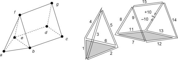
FIGURE 4.33 A spatial subdivision (left) combining a tetrahedron with a wedge, and a sketch (right) of its combinatorial map; only edge 10 is represented by two darts.
[S,σ1,…, ση](n ≥ 2) is an n-dimensional combinatorial map iff S is a finite set;σ1 is a permutation of S; and σ2,…, ση are involutions on S such that σi º is an involution on S for 1 ≤ i ≤ n − 2 and i + 2 ≤ j ≤ n. For example, in 3D, σ1 ºσ3 is an involution on S. In 2D, we had σ1 = θ and σ2 = σ; the additional condition is vacuous.
Figure 4.33 shows a spatial subdivision. Let the following be given:

These permutations define a 3D combinatorial map on a set S of 30 darts.
In general, let {θ1,…, θm} be a set of permutations defined on a set S. A dart e ∈ S and a permutation θ of S define a cycle θ(e) of darts that are “reachable ” by starting at e and using only transitions contained in θ. For example, for the σ1,σ2, and σ3 defined above, we have σ1 ![]() σ2(12) = (12, 13, − 11, 7) and σ3
σ2(12) = (12, 13, − 11, 7) and σ3 ![]() σ1
σ1 ![]() σ2(−6) = (−6,6). The orbit of a dart e is the set of all darts contained in cycles θ(e), where θ is any finite sequence of permutations θi or
σ2(−6) = (−6,6). The orbit of a dart e is the set of all darts contained in cycles θ(e), where θ is any finite sequence of permutations θi or ![]() . For example, the orbit of a dart with respect to σ1,σ2, and σ3 is either the set of all darts of the tetrahedron or the set of all darts of the wedge.
. For example, the orbit of a dart with respect to σ1,σ2, and σ3 is either the set of all darts of the tetrahedron or the set of all darts of the wedge.
3D combinatorial maps can be used to represent spatial subdivisions. For example, merging the tetrahedron and wedge shown in Figure 4.33 means deleting the doubly represented face between them; similarly, splitting can be done by creating new separating faces. Spatial segmentation can be based on repeated merging operations that reduce the total number of darts.
4.5 Exercises
1. Show that EM ⊆ OM ⊆ M ⊆ CM ⊆ DM for any M ⊆ S.
2. Show that E and D are dual operations (i.e., that ![]() for any M ⊆ S) where
for any M ⊆ S) where ![]() .
.
3. Show that O and C are idempotent operations (i.e., that O2M =OM and C2M = CM for any M ⊆ S).
4. Prove that the center of a simply 4-connected set of grid points, using the graph distance defined by A4, is either a 2 × 2 square, a diagonal line segment, or a diagonal staircase; note that, in the latter two cases, the center can contain arbitrarily many grid points (see Figure 4.12). What happens if we use A8∈
5. Eulerian paths can be defined for an infinite graph provided it is connected and its set of edges is countably infinite. P. Erdös, T. Grünwald, and E. Vàzsonyi [308] showed in 1938 that an infinite Eulerian path can be either of the following:
(i) one-way (i.e., with one terminal node) if at most one node of the graph has odd degree; if no node has odd degree, there must be at least one node of infinite degree, and the complement of any finite subgraph must have only one infinite component; or
(ii) two-way (i.e., with no terminal node) if no node has odd degree; the complement of any finite subgraph has at most two infinite components; and any finite subgraph that contains only nodes of even degree has only one infinite component.
Consider the three infinite graphs in Exercise 1 in Section 1.3. Do they have Eulerian paths? If so, are they one-way or two-way?
6. Do the 4-adjacency grids Gn,n (n ≥ 2) have Hamiltonian circuits? Do they have Hamiltonian paths?
7. Find a Hamiltonian path for the infinite 4-adjacency grid [Z2,A4].
8. Show that the following two graphs are isomorphic:

9. Is this graph planar? Verify your answer.

10. Let P be a picture with values in {0,…, Gmax}. Define a relation AP on the set of pixels of P using the following:
Is the graph [S,AP] connected? complete? planar? Eulerian?
11. Show that any local circular order on K3,3 or K5 (see Figure 4.32) results in an oriented graph that has the Euler characteristic χ+ < 2.
12. The solid dots in the following figure are the grid points in a subset M of the infinite 4-adjacency graph [Z2,A4]. Draw the region adjacency graph of M. Calculate the Euler characteristics of the components of this graph assuming clockwise orientation ((A) in Figure 4.19).

13. Can a finite oriented adjacency graph have α0 = α1 = α2?
14. A complete graph G with α0 nodes has α1 = α0(α0 − 1)/2 edges. If α0 ≥ 3, prove that, for any local circular order on G, we have χ+ ≤−α0(α0 −7)/6.
15. Specify permutations of 2D combinatorial maps that represent the following 8-adjacency graphs:
![]()
16. Let L, M ⊆ S be subgraphs of the graph [S, A]. Show that p ∈ δ(L ⊆ M) or p ∈ δ(L ∩ M) implies that p ∈ δ(L) or p ∈ δ(M). Furthermore, if p ∈ δ(L) and M ⊆ S, then either p ∈ ⊆ M) or p ∈ δ(L ∩ M).
17. Let L, M be subgraphs of a finite graph [S, A]. Define Q(L, M) as the set of all nodes p ∈ δ(L) ∩δ(M) that are not in δ(L ⊆ M). Prove the following:
18. Let L be a subgraph of a subgraph M of a graph [S,A], and let δs(M) denote the border of M. Prove the following:
Also, prove the following for all p ∈ S:
19. A subset M of a graph G =[S, A] is called a D-cluster (D ≥ 1) iff, for all p, q ∈ M, there exists a sequence p = p0, p1,…, pn = q of nodes in S such that dG (pi−1,pi) ≤ D (i = 1,…, n). (Here dG is the graph metric, in which each edge has unit length; it follows that M is a 1-cluster iff it is connected.) The D-hull HD (M) of M is the set of nodes of G within distance D/2 of M. The geodesic D-hull GD (M) of M
is the set of nodes of G that lie on shortest paths of length ≤ D between pairs of nodes of M. Prove that M is a D-cluster iff HD(M) is connected iff GD (M) is connected.
4.6 Commented Bibliography
Region adjacency graphs on regular grids were introduced in [151, 881]. The notions of connectedness and components as used in graph theory had to be adapted to the special needs of picture analysis by defining connectedness with respect to a subgraph. For information about using “local properties ” to compute topologic properties of pictures, see [377, 377]. Exercise 19 is from [889], which also defines “D-holes ” and “D-borders ” for sparse sets of 1s in binary pictures. [574, 1109] initiated studies of general adjacency models in picture analysis.
The history of graph theory is reviewed in [862]. There are many textbooks about graph theory; see, for example, [786], which is the source of Exercise 3, and [1073], which is the source of Exercises 16, 17, and 18. Periodic subgraphs of the infinite 8-adjacency graph on Z2 are studied in [1070]. For graph algorithms, see [997]. For Steinitz’s theorem, see [1026]; for Kuratowski’s theorem, see [611].
I. Lakatos’s book of dialogues [614] (published after he died in 1974) discusses the very diverse opinions about polyhedra that do not obey the Descartes-Euler polyhedron theorem that were expressed by many mathematicians, including Legendre, Gergonne, Cauchy, Lhuilier, Crelle, Hessel, Becker, Listing, Möbius, Schlä;fli, Grunert, Becker, Poinsot, Steiner, Hoppe, de Jonquières, Matthiessen, Poincaré, Hilbert, Steinhaus, Pólya, and Forder. For example, in 1852, L. Schlä;fli [962] declared about Kepler’s urchin9 that “this is not a genuine polyhedron, for it does not satisfy the condition V – E + F = 2”!
Theorem 4.2 is from [886]. In general, let P be an n-dimensional binary picture defined on a finite hypercuboidal (2n, 3n − 1)- or (3n −1, 2n)-adjacency grid that is extended into Zn; then the region adjacency graph of P is a tree [502].
Dijkstra’s algorithm was independently discovered in [1124]. The application of shortest path algorithms to picture analysis is discussed in [452, 1095]. Exercise 7 is from [507]. For the complexity of algorithms and computational problems (e.g., NP-completeness), see [356]. For efficient planarity tests, see [443]. [687] discusses components in 2D and 3d adjacency grids that have uniquely defined Hamiltonian circuits. For centers of graphs defined by 4- or 8-regions, see [247] and [507].
The directional code introduced by H. Freeman [342] can be regarded as an example of an orientation on an adjacency graph. Oriented adjacency graphs were studied in a series of publications in the 1980s (e.g., [553, 1104, 1111]). Theorems 4.6 and 4.7 are from [1111]. Border tracing can also be defined in picture data structures such as quadtrees [290]. The book [65] provides an overview of curve tracing methods in picture analysis. The formula in Exercise 14 is proved in [1104]. Many of the combinatorial results about the Gv,λs in Section 4.3.7 are from [1103].
The theory of combinatorial maps was initiated by L. Heffter at the end of the 19th century [415]. He introduced maps and proved a dual characterization theorem for them. Maps were used, for example, by G. Ringel starting in the 1950s, were reinvented in [301, 1153], and finally became popular in discrete mathematics [383]. Their relevance for modeling 2D or 3D (segmented) pictures is discussed in [82, 117, 287, 326, 651, 959].
1In graph theory, nodes are often called vertices, and edges are sometimes called arcs. To avoid confusion with grid vertices, we will use the term “node.”
2The abstract representation of the Königsberg bridges in Figure 1.15 is not a graph, because it has multiple “edges ” between some pairs of nodes. In such a multigraph, R is a “bag ” (a “set ” in which elements can be repeated) of pairs of nodes.
4A computational problem is called NP-complete iff it is both NP (solvable in nondeterministic polynomial time) and NP-hard (any other NP problem can be translated into it) [356]. Algorithms that solve NP-complete problems have time complexities that may be between polynomial and exponential, exponential (e.g., using exhaustive search), or even bigger than exponential (e.g., on the order of nn). “Approximate ” solutions to NP-complete problems can sometimes be found that have lower computational cost.
5This is an informal definition; a formal definition will be given in Section 4.3.2.
6This formula appeared in an earlier (unpublished) fragment by R. Descartes; it is sometimes called the Descartes-Euler polyhedron theorem. It was discovered by L. Euler (1707–1783) around 1750 for convex polyhedra and was first proved in 1794 by A.-M. Legendre (1752–1833).
7Georg Pick was a professor of mathematics in Prague. He was in close contact with A. Einstein when Einstein worked at Prague University in 1911 and 1912. They played music together, discussed philosophy, and established the mathematic basis of general relativity theory. Pick was murdered by the Nazis in the Theresienstadt concentration camp.
8In this example, 1 goes into − 1 in σ, − 1 goes into 2 in θ (1 goes into 2 in θ ºσ), 2 goes into −2 in σ, −2 goes into − 7 in θ (2 goes into − 7 in θ ºσ), and so on.
9Also “echinus,” which is Kepler’s original name for the small stellated dodecahedron that has 12 faces, each a regular star pentagon. It is one of the Kepler-Poinsot solids with the dual polyhedron (see the end of Section 4.2.2) that is the great dodecahedron [220, 614]; for both, we have α0 −α1 +α2 = −6.