
Morphologic Operations
Mathematic morphology deals with operations that replace the value of a pixel p with the max or min of the values of a set of neighbors of p. This chapter introduces dilation and erosion operations as well as combinations of such operations known as hit-and-miss transforms and opening and closing operations. It illustrates how such operations can be used to simplify a picture (e.g., to remove “noise” from it) or to decompose or “segment” it into parts.
The primary subject of this chapter is the study of operations on a picture that replace the value of each pixel p with the maximum (or the minimum) of the values of a set of neighbors of p. (Such operations were briefly introduced in Section 1.2.12 and were also used in Sections 4.1 and 12.2.3.) If the picture is binary (its pixel values are all 0s and 1s), such a “local maximum” operation has the effect of “dilating” the 1s; p ’s value becomes (or remains) 1 if any of its neighbors (that belong to the specified set) had value 1. Similarly, a local minimum operation has the effect of dilating the 0s. Note that dilating the 1s is equivalent to “eroding” the 0s, and dilating the 0s is equivalent to eroding the 1s. Evidently, dilation is quite different from magnification (which “expands” both the 1s and the 0s), and erosion is quite different from demagnification (which “contracts” both the 1s and the 0s.)
Dilation and erosion (and the other operations discussed in this chapter) are defined for multivalued pictures, but they have simple geometric interpretations when they are applied to binary pictures. These operations are therefore usually called morphologic operations; morphology is the study of form and pattern (i.e., of geometric properties of binary pictures). We will define the concepts in this chapter only for 2D pictures, but they generalize straightforwardly to higher dimensions.
15.1 Dilation
Let σ be a nonempty set of pixels at locations specified relative to an origin o. For any pixel p, the σ-neighborhood σ (p) of p is the set of pixels that coincide with the pixels of σ when they are translated so that o coincides with p. Evidently,σ(p) = {p + s : s ∈ σ} where + denotes coordinate-wise addition ((x,y) + (u,v) = (x + u,y + v)). Note that o is not necessarily in σ, so p may not be in its own σ-neighborhood. We will assume from now on that σ is finite. In mathematic morphology (the standard name for the subject of this chapter),σ is usually called a structuring element.
Definition 15.1
Let P (p) be the value of the pixel p in the picture P. The σ-dilation P(σ) of P is the picture in which the following is true:
If o ∈ σ, we have p ∈ σ (p) so that maxq∈σ(p)P(q) ≥ P(p). Thus, if o ∈ σ, we have P(σ) ≥ P at every pixel p; however, this is not true if o ∉σ.
If P is a binary picture, P(σ) is evidently also a binary picture. Moreover, P(σ) (p) = 1 iff P(q) = 1 for some pixel q of σ (p). Let (P) denote the set of pixels of P that have value 1; then ![]() . Using the notation of set-theoretic mathematic morphology (see Section 1.2.12), we have
. Using the notation of set-theoretic mathematic morphology (see Section 1.2.12), we have ![]() .
.
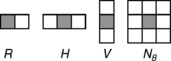
Evidently, if σ = {o}, we have P(σ) = P; in general, if σ is a single pixel in some location (x, y) relative to o, then P(σ) is the result of translating P by (–x, –y). The term “dilation” is more appropriate if σ is a set of two or more pixels that contains o. For example (see Figure 15.1), if σ = R consists of the pixels in locations (0,0) (the location of o) and (0,1),P(σ) is obtained by “smearing” the values of P toward the left; the value of p in P(σ) is the max of the values of p and its righthand neighbor. Similarly, if σ = H consists of o and its two horizontal neighbors, P(σ) is obtained by “smearing” the values of P to the right and left; if σ = V consists of o and its two vertical neighbors, P(σ) is obtained by “smearing” P up and down; and if σ = N8 is the 8-neighborhood of o (the set consisting of o and its horizontal, vertical, and diagonal neighbors), P(σ) is obtained by “smearing” P horizontally, vertically, and diagonally. Note that, in these last three cases,σ is symmetric about o.
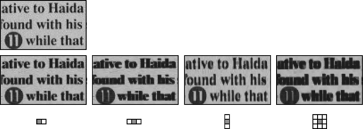
The results of dilating some simple binary pictures (1s = black, 0s = white)1 using the four σs in Figure 15.1 are shown in Figure 15.2. Analogous results for a picture of some text (in which dark pixels have high values) are shown in Figure 15.3.

FIGURE 15.2 Dilations of a set of binary pictures (shown in the left column) using the four structuring elements shown in Figure 15.1. Note that “object” pixels (which have value 1) are displayed as black. The pixels added by the dilations are shown in gray.
15.2 Erosion
If o ∈ σ, we have p ∈ σ (p),so minq∈σP(p)P(q) ≤ P (p) (i.e., P(σ) ≤ P).
If P is a binary picture, so is P(σ). Moreover, P(σ) (p) = 1 iff P(q) = 1 for every pixel q of σ(p); in other words, ![]() in the notation of Section 1.2.12
in the notation of Section 1.2.12
Evidently, if σ is a single pixel in location (x, y),P(σ) is the same as P(σ) (i.e., it is the result of translating P by (–x, –y)). The term “erosion” is more appropriate if σ is a set of two or more pixels that contains o.
The results of eroding the binary pictures shown in Figure 15.2 using the four structuring elements in Figure 15.1 are shown in Figure 15.4, and the results of eroding the text picture of Figure 15.3 using these structuring elements are shown in Figure 15.5. Note that, in these pictures, dark pixels have high values (in the binary pictures, object pixels have value 1), so erosion removes object pixels.

FIGURE 15.4 Erosions of the same set of binary pictures as shown in Figure 15.2 using the same four structuring elements. Note that “object” pixels (value 1) are displayed as black. The pixels deleted by the erosions are shown in light gray.
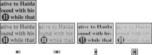
FIGURE 15.5 Erosion of the text picture (the same one as was used in Figure 15.3) using the same four structuring elements. Note that dark pixels have high values.
Dilations and erosions commute with monotonic transformations of the pixel values of a picture P. Indeed, let P* be a picture obtained from P by applying a monotonic function f to the pixel values of P so that, for any pixel p, we have P* (p) = f (P(p)). p has value maxq∈σ(p)P(q) in P(σ) and value maxq∈σ(p)P* (q) = max q∈σ(p)f (P(q)) in P*(σ). Because f is monotonic, both maxima are taken on at the same pixel(s) q; hence, the second maximum is f of the first maximum. Thus, dilating a picture and then applying a monotonic transformation to its pixel values gives the same result as applying the monotonic transformations and then dilating the picture; this is similar for erosion.
15.3 Combining Dilations and Erosions
In this section, we discuss two methods of combining dilations and erosions:
a) hit-and-miss transforms, which dilate and erode a picture using disjoint structuring elements; and
b) opening and closing operations, which erode a picture and then dilate it (or vice versa) using the same structuring element (which we assume to be symmetric and to contain o).
15.3.1 Hit-and-miss transforms and templates
Let P be a binary picture and let σ and τ be two structuring elements. We have seen that P(σ) (p) = 1 iff P = 1 at every pixel of σ(p). Similarly, ![]() iff
iff ![]() (i.e., P = 0) at every pixel of τ(p).
(i.e., P = 0) at every pixel of τ(p).
Definition 15.3
![]() is called the hit-and-miss transform of P by the pair of structuring elements (σ, τ).
is called the hit-and-miss transform of P by the pair of structuring elements (σ, τ).
Hit-and-miss transforms can be used to identify pixels of P with neighborhoods that have 1s in specified locations (defined by σ) and 0s in specified locations (defined by τ). For example, if σ = {(0,0)} and τ = {(0,1)}, then p = 1 in ![]() iff, in P, we have p = 1 and q = 0 where q is the upper neighbor of p. Evidently, if σ and τ intersect,
iff, in P, we have p = 1 and q = 0 where q is the upper neighbor of p. Evidently, if σ and τ intersect, ![]() must be identically zero, because we can never have both P(σ)(p) = 1 and
must be identically zero, because we can never have both P(σ)(p) = 1 and ![]() ; hence, we can assume that σ and τ are disjoint. We can think of σ and τ as defining a “template” in which the pixels of σ are 1s and the pixels of τ are 0s; evidently, we have min
; hence, we can assume that σ and τ are disjoint. We can think of σ and τ as defining a “template” in which the pixels of σ are 1s and the pixels of τ are 0s; evidently, we have min ![]() iff the neighborhood of p “matches” this template. Mathematic morphologists also use the notation
iff the neighborhood of p “matches” this template. Mathematic morphologists also use the notation ![]() for the hit-and-miss transform
for the hit-and-miss transform ![]() of
of ![]() . It follows that
. It follows that ![]() .
.
If P is multivalued, a hit-and-miss transform can be used to identify pixels with σ-neighbors that have high values and with τ-neighbors that have low values. Let ![]() be the picture in which
be the picture in which ![]() for all p; then
for all p; then ![]() has a high value iff the σ-neighbors of p have high values and its τ-neighbors have low values. In Section 15.5, we will give examples of the use of binary hit-and-miss transforms to detect local features in a picture. Unlike dilation, erosion, opening, and closing, the hit-and-miss transform is uniquely defined for binary pictures only. See [874, 1012] for alternative definitions of hit-and-miss transforms for multivalued pictures. [1012] applies structuring elements (σ,τ) to different “layers” (binary pictures defined by thresholds) of a multivalued picture.
has a high value iff the σ-neighbors of p have high values and its τ-neighbors have low values. In Section 15.5, we will give examples of the use of binary hit-and-miss transforms to detect local features in a picture. Unlike dilation, erosion, opening, and closing, the hit-and-miss transform is uniquely defined for binary pictures only. See [874, 1012] for alternative definitions of hit-and-miss transforms for multivalued pictures. [1012] applies structuring elements (σ,τ) to different “layers” (binary pictures defined by thresholds) of a multivalued picture.
15.3.2 Opening and closing
Let σ be a structuring element that is not necessarily symmetric. (We recall that it is symmetric iff ![]() , where
, where ![]() denotes the mirror set.)
denotes the mirror set.)
Definition 15.4
Dilating a picture P by σ and then eroding it by ![]() (i.e., constructing the picture
(i.e., constructing the picture ![]() is called σ-closing. Similarly, eroding P by σ and then dilating it by
is called σ-closing. Similarly, eroding P by σ and then dilating it by ![]() (i.e., constructing
(i.e., constructing ![]() is called σ-opening.
is called σ-opening.
For binary pictures, opening by σ transforms ![]() into the union of all translates of σ that are contained in
into the union of all translates of σ that are contained in ![]() . Closing of
. Closing of ![]() by σ is the same as opening
by σ is the same as opening ![]() by σ.
by σ.
Proof We prove the inequality for opening; the proof for closing is similar. Eroding 〈P〉 by σ and then dilating by ![]() gives the following:
gives the following:
For every q in ![]() , p is in σ(q), so min{P (r): r ∈ σ (q)} is ≤ P (p), and, because this is true for all such q, its maximum over
, p is in σ(q), so min{P (r): r ∈ σ (q)} is ≤ P (p), and, because this is true for all such q, its maximum over ![]() . Hence,
. Hence, ![]() .
.
If P is a binary picture, we recall that ![]() is the union of σ(p) for all
is the union of σ(p) for all ![]() , and
, and ![]() is the set of all p such that
is the set of all p such that ![]() . It follows that
. It follows that ![]() is the union of the σ(p)s that are contained in
is the union of the σ(p)s that are contained in ![]() . The result of σ-closing a binary picture can be characterized similarly. In Sections 15.4 and 15.6, we will show how opening and closing operations can be used to simplify or “segment” a (not necessarily binary) picture.
. The result of σ-closing a binary picture can be characterized similarly. In Sections 15.4 and 15.6, we will show how opening and closing operations can be used to simplify or “segment” a (not necessarily binary) picture.
15.4 Simplification
In this section, we will show how opening and closing operations can be used to “simplify” or “smooth” a picture by eliminating minor irregularities in its pixel values —in particular, by eliminating small (more precisely, thin) groups of high-valued pixels from a region of low-valued pixels or vice versa. Such irregularities may result if random changes are made in the pixel values.2 In a smooth region of a picture (i.e., a region in which the values of adjacent pixels are the same or differ only slightly; see Section 14.4), random changes will produce many pixels with values that differ significantly from those of their neighbors, because the changes are unlikely to have the same effect on the pixel and its neighbors. Similarly, along an edge in a picture (a smooth locus of large changes in pixel values; e.g., when a high-valued region is adjacent to a low-valued region along a smooth frontier), random changes of pixel values from high to low and vice versa will produce irregularities in the edge.
A picture is said to contain salt-and-pepper noise if low-valued pixels occasionally occur in regions of high-valued pixels and vice versa. (Recall that, in this chapter, low values are light and high values are dark.) “Salt” can be eliminated by dilating the picture and “pepper” by eroding it, provided we use a structuring element σ such that the exceptional pixels always have nonexceptional σ-neighbors. However, dilation enlarges dark regions and erosion shrinks them (and vice versa for light regions), so dilation or erosion distorts the picture. We will now show how to eliminate salt or pepper but avoid enlarging the dark or light regions by eroding and then dilating (i.e., opening) or dilating and then eroding (i.e., closing).
Figure 15.6 shows, on the left, a picture P that contains a dark object on a light background. The values of some of the pixels of P have been complemented (i.e., value w has been occasionally replaced by Gmax – w); this results in salt-and-pepper noise. Closing P (using the structuring element N8; see Figure 15.1, right) eliminates the “salt” but does not enlarge the object; similarly, opening P using N8 eliminates the “pepper” but does not shrink the object. These effects are also illustrated in Figure 15.7 for a larger (binary) picture; note that clusters of noise pixels are often not eliminated.

FIGURE 15.6 Removing “salt-and-pepper” noise by opening and closing. From left to right: original picture (note that dark pixels have high values); picture with noise; closing with N8; opening with N8.

FIGURE 15.7 Left: noisy binary picture P; note that black pixels have value 1. Center: result of closing P using N8. Right: result of opening P using N8.
Opening eliminates not only isolated high-valued pixels but also “thin” sets of high-valued pixels, and closing eliminates not only isolated low-valued pixels but also “thin” sets of low-valued pixels. Specifically, we call a set S of pixels σ-thin if every pixel of S has σ-neighbors in the complement ![]() of S. If S consists of light pixels and
of S. If S consists of light pixels and ![]() of dark pixels and S is σ-thin, σ-erosion eliminates all of the light pixels that were in S. Subsequent
of dark pixels and S is σ-thin, σ-erosion eliminates all of the light pixels that were in S. Subsequent ![]() -dilation cannot replace these light pixels, because the pixels of
-dilation cannot replace these light pixels, because the pixels of ![]() are all dark; hence, σ-opening eliminates S. Similarly, if S consists of dark pixels and
are all dark; hence, σ-opening eliminates S. Similarly, if S consists of dark pixels and ![]() of light pixels and S is σ-thin, σ-closing eliminates S. Thus, opening or closing should not be applied to a picture if it contains thin light or dark regions such as lines or curves that are significant (i.e., that are not merely “noise”).
of light pixels and S is σ-thin, σ-closing eliminates S. Thus, opening or closing should not be applied to a picture if it contains thin light or dark regions such as lines or curves that are significant (i.e., that are not merely “noise”).
To illustrate how opening eliminates thin sets of high-valued pixels, let P be a binary picture and let σ be N8. Suppose ![]() where U is a square of size of at least 3 × 3 and V is a rectangle of width 2 so that V is N8-thin.
where U is a square of size of at least 3 × 3 and V is a rectangle of width 2 so that V is N8-thin. ![]() contains U, because every pixel of U is contained in a 3 × 3 square that is contained in
contains U, because every pixel of U is contained in a 3 × 3 square that is contained in ![]() ; however, it does not contain any pixel of V, because no pixel of V is contained in a 3 × 3 square that is contained in
; however, it does not contain any pixel of V, because no pixel of V is contained in a 3 × 3 square that is contained in ![]() . On the left side of Figure 15.8, the top picture is P; in the middle picture, the pixels of
. On the left side of Figure 15.8, the top picture is P; in the middle picture, the pixels of ![]() are black, and the remaining pixels of
are black, and the remaining pixels of ![]() are light gray; in the bottom picture, the pixels of
are light gray; in the bottom picture, the pixels of  are black or dark gray. We see that N8-opening of P eliminates V but leaves U intact. A less trivial example is shown on the right side of Figure 15.8. We see that the “thick” parts of the object have survived but the thin parts have been eliminated; as a result, the shapes of the surviving thick parts have been simplified.
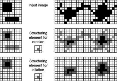
FIGURE 15.8 Two examples of how opening can be used to eliminate thin parts of an object. Note that object pixels are black. In the second row, pixels of ![]() are black, and the remaining pixels of
are black, and the remaining pixels of ![]() are light gray. In the third row, pixels of
are light gray. In the third row, pixels of ![]() are black or dark gray.
are black or dark gray.
Similarly, closing adjoins to ![]() thin parts of the complement of
thin parts of the complement of ![]() . For example, let
. For example, let ![]() , where U is a square and V a rectangle within U of sizes as in the preceding paragraph, as illustrated on the left of Figure 15.9. Then
, where U is a square and V a rectangle within U of sizes as in the preceding paragraph, as illustrated on the left of Figure 15.9. Then  contains V, because every pixel of V is contained in a 3 × 3 square that is centered at a pixel of U – V. A less trivial example is shown on the right of Figure 15.9.

FIGURE 15.9 Two examples of how closing can be used to eliminate thin parts of the complement of an object: (top) P; (bottom) (P(σ))(σ). Note that object pixels are black.
In these examples, the thin regions are N8-thin (i.e., they are not more than two pixels thick). In general, “thin” regions can be arbitrarily thick, but they can be eliminated from or adjoined to a set by performing an opening (or closing) operation that uses a sufficiently large structuring element; see Section 15.6. The pictures in these examples are binary, but the same methods can be applied to multivalued pictures to eliminate thin parts of dark (or light) objects or to adjoin to them thin parts of their background.
15.5 Segmentation
This section discusses ways of defining distinctive sets of pixels in a picture. Partitioning a picture into distinctive subsets is called segmentation. We briefly describe some basic methods of segmentation, with emphasis on their relationship to morphologic operations. Segmentation is treated extensively in books about picture processing and computer vision (e.g., segmentation of a picture into “watersheds” was discussed in Section 13.3.3).
15.5.1 Thresholding
If a subset S of the pixels in a picture P has values that differ significantly from those of (most of) the other pixels of P, we call S distinctive. For example, if the pixels of S have significantly higher values than the other pixels, we can choose a threshold t such that pixels with values of t or greater (almost all) belong to S. We can then define a binary picture Pt in which Pt(p) = 1 iff P(p) ≥ t. This process of converting a multivalued picture into a binary picture by comparing its pixel values to a threshold is called thresholding. Some simple examples of thresholding are shown in Figure 15.10.

FIGURE 15.10 Original picture (as seen in Figure 15.6) and results of thresholding it using thresholds 115, 204, and 232 (from left to right).
Evidently, thresholding a picture P is a monotonic transformation of the pixel values of P. It follows (see Section 15.2) that dilations and erosions commute with thresholding. Thus, dilating or eroding a picture and then thresholding it has the same effect as thresholding the picture and then dilating or eroding the resulting binary picture. Similarly, because opening is erosion followed by dilation and closing is dilation followed by erosion, these operations also commute with monotonic transformations of the pixel values and, in particular, with thresholding; thus, opening or closing a picture and then thresholding it has the same effect as thresholding the picture and then opening or closing the resulting binary picture.
More generally, a picture can be segmented using two (or more) thresholds [l,h] (0 ≤ l <h ≤ Gmax); all pixels with values u that are between l and h are kept, and all those with values that are < l or > h are rejected. See [557] for other methods of binarizing multivalued pictures.
15.5.2 Local features
A pixel p of P is said to belong to a local feature in P if the neighbors of p have a distinctive pattern of values. For example, p (e.g., at (x,y)) lies on a vertical edge if a set of its neighbors on the right (e.g., (x + 1, y + 1), (x + 1, y), and (x + 1, y−1)) has high values and a set of its neighbors on the left (e.g., (x − 1, y + 1), (x − 1, y), and (x − 1, y−1)) has low values, or vice versa. Similarly, the pixel at (x, y) lies on a vertical line if the pixels at (x,y + 1), (x, y), and (x,y −1) have high values and the pixels at (x − 1, y + 1), (x − 1, y), (x − 1, y −1), (x + 1, y + 1), (x + 1, y), and (x + 1, y −1) have low values or vice versa. Edges and lines in other directions are defined analogously. “Spots” are pixels with values that are higher (or lower) than those of all of their adjacent pixels.
Pixels that belong to local features can be identified using hit-and-miss transforms. For example, pixels that lie on a vertical edge in a binary picture P can be identified by eroding P using σ = {(1,1), (1,0), (1,-1)} and dilating P using σ = {(−1,1), (−1,0), (−1,−1)} (or vice versa) and taking the min of the results. Even if P is not binary, the value of this min will be high at p iff p lies on a vertical edge. Examples of the use of hit-or-miss transforms to identify spots and “notches” in horizontal lines are shown in Figure 15.11.

15.5.3 Texture
The texture of a region in a picture can be characterized by the presence of many pixels that belong to local features of particular types. For example, the texture is “spotted” if the region contains many spots, “busy” if it contains many edges, “striped” if it contains many lines, and “directional” if the edges or lines all have similar directions.
In general, when such hit-and-miss transforms are applied to a picture, regions of the picture that contained many occurrences of specific local features will contain many high-valued pixels. In Section 15.6, we will describe a method of finding regions of a picture that contain many high-valued pixels.
Texture is discussed extensively in books about picture analysis and computer vision. In this book, we do not discuss signal-theoretic, statistic, or perceptual approaches to texture characterization.
15.6 Decomposition
The segmentation methods described in Section 15.5 used individual pixel values or local patterns of pixel values to identify distinctive pixels. In this section, we describe methods of segmenting a picture into parts that are characterized by geometric properties. These methods make use of morphologic operations in which the structuring elements can be of arbitrary size. To distinguish these methods from segmentation methods based on individual or local pixel values, we call them decomposition methods.
Let σh be the structuring element that consists of the pixels that have distances from the origin (using any desired metric) that are at most h> 0. For example, if we use the metric d8, σ1 is N8. Note that σh is symmetric and contains o. We will abbreviate σh by h in superscripts and subscripts (e.g., the σh-dilation of P will be denoted by P(h)).
15.6.1 Clusters
We first show how to use closing to “fuse” a cluster of high-valued pixels (i.e., a large number of such pixels in a region R made up of other pixels that have low values) so that, after the closing, all of the pixels of R have high values. The basic idea is that, if the pixels in the cluster are at distances less than 2h from each other, the sets of low-valued pixels between the cluster pixels are σh-thin. As we saw in Section 15.4, closing can be used to adjoin to a set S thin parts of the complement of S. Hence, closing can be used to adjoin to the cluster pixels the thin sets of low-valued pixels between the cluster pixels so that all of the pixels of R are adjoined to the cluster.
Figure 15.12 shows simple examples of how eliminating thin parts of ![]() can be used to fuse a cluster of dark pixels of
can be used to fuse a cluster of dark pixels of ![]() . If S is a cluster, any pixel of
. If S is a cluster, any pixel of ![]() that is “surrounded” by pixels of S belongs to a thin part of the complement
that is “surrounded” by pixels of S belongs to a thin part of the complement ![]() . The closing adjoins these thin parts to S and thus fuses S into a solid region. The picture in this example is binary, but the example generalizes straightforwardly to multivalued pictures and to sparser clusters (i.e., those that use larger structuring elements).
. The closing adjoins these thin parts to S and thus fuses S into a solid region. The picture in this example is binary, but the example generalizes straightforwardly to multivalued pictures and to sparser clusters (i.e., those that use larger structuring elements).

15.6.2 Elongated object parts
Closing with structuring elements of different sizes can be used to segment a picture into clusters (of high-valued pixels on a low-valued background) that have different densities. Similarly, opening with structuring elements of different sizes can be used to eliminate thin high-valued regions that have different thicknesses.
Figure 15.13 shows a binary picture P that contains sets of 1s that have different thicknesses and the results of opening P using the structuring elements σ1, σ2, and σ4. (These structuring elements are squares of sizes 3 × 3, 5 × 5, and 9 × 9; they are the sets of pixels with d8-distances from o that are ≤ 1, ≤ 2, and ≤ 4. Such a sequence of openings by balls of increasing diameter is called a granulometry in mathematic morphology [706, 969].) The σ1-opening eliminates the thinnest sets of 1s; the σ2-opening eliminates thicker sets of 1s; and the σ4-opening eliminates all but the thickest sets of 1s. Another example is shown in Figure 15.14; here, the sets of high-valued pixels do not have constant thicknesses, but they can be almost entirely eliminated by opening using a structuring element of the appropriate size.
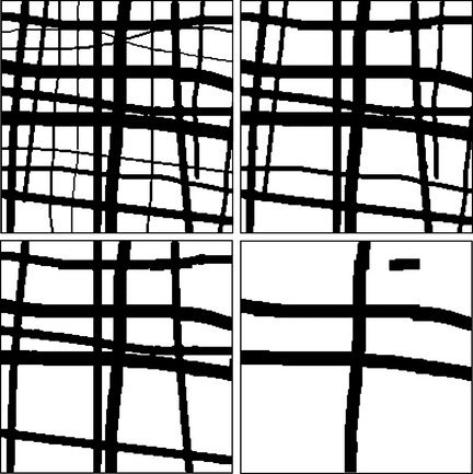
FIGURE 15.13 An example of how opening can be used to detect and eliminate sets of object pixels that have various thicknesses. Note that object pixels are black. Upper left: original object. Remaining pictures: results of opening using square structuring elements of sizes 3 × 3, 5 × 5, and 9 × 9.

FIGURE 15.14 Opening of a thresholded aerial picture (upper left) using structuring elements of different sizes.
Opening using structuring elements of increasing sizes can be used to identify elongated sets of high-valued pixels in a picture. Let P be a binary picture, and let ![]() be the set of 1s of P that remain after opening
be the set of 1s of P that remain after opening ![]() using an h × h structuring element. Thus,
using an h × h structuring element. Thus, ![]() consists of “h-thick” parts of
consists of “h-thick” parts of ![]() (i.e., parts of which every pixel is contained in an h × h square that is contained in
(i.e., parts of which every pixel is contained in an h × h square that is contained in ![]() ). This fact can be used to identify elongated parts of
). This fact can be used to identify elongated parts of ![]() that have thickness of at most h. Suppose we call an h × k rectangle “elongated” if k ≥ 3h. Then a connected component of
that have thickness of at most h. Suppose we call an h × k rectangle “elongated” if k ≥ 3h. Then a connected component of ![]() that contains at least 3h2 pixels must have been an elongated part of
that contains at least 3h2 pixels must have been an elongated part of ![]() having a thickness of less than h. For example, the sets of pixels in Figure 15.13 that are eliminated by σi-opening (i = 1,2,4) have 819, 2829, and 9681 pixels, respectively, so they are all elongated. Similarly, in Figure 15.14, the sets of pixels that are eliminated by σi-opening (i = 1,2,3) have 7824, 10,020, and 14,042 pixels, respectively, and so are all elongated.
having a thickness of less than h. For example, the sets of pixels in Figure 15.13 that are eliminated by σi-opening (i = 1,2,4) have 819, 2829, and 9681 pixels, respectively, so they are all elongated. Similarly, in Figure 15.14, the sets of pixels that are eliminated by σi-opening (i = 1,2,3) have 7824, 10,020, and 14,042 pixels, respectively, and so are all elongated.
An alternative method of detecting elongated sets is to use the union of openings by elongated structuring elements in all (main) directions.
15.6.3 Distance transforms and medial axes
We conclude this section by showing how morphologic operations can be used to compute distance transforms (see Section 3.4.2) and medial axes (see Section 3.4).
Let P be a binary picture, let P(0) = P, and let P(i+1) be the result of eroding P(i) (i = 0,1,…, D−1) using the structuring element H ∪ V or N8 (see Figure 15.1), where D is the diameter of P. Then ![]() is the distance transform of P; using H ∪ V gives the d4 transform, and using N8 gives the d8 transform.
is the distance transform of P; using H ∪ V gives the d4 transform, and using N8 gives the d8 transform.
Let P(i) be as in Proposition 15.2, and let P(i)* be the result of redilating P(i) (once) using the same structuring element that was used in the erosions. Thus P(i)* is an opening of P(i-1) so that, in accordance with Proposition 15.1, P(i)* ⊆P(i-1). Then ![]() .
.
Note that this method of constructing the medial axis can also be applied to multivalued pictures.
15.7 Exercises
1. If σ = {(x1, y1),…, (xn, yn)}, prove that P(σ) is the max of the translates of P by (–χ1,–y1),…, (–χn, – yn).
2. Let H = {(−1,0), (0,0), (1,0)} and V = {(0, −1), (0,0), (0,1)}, and let E = N8 consist of (0,0) and its eight horizontal, vertical, and diagonal neighbors. Prove the following:
3. Let ![]() denote the reflection of σ in the origin (i.e., {(-x, -y): (x, y) ∈σ}). If σ is symmetric, we have σ =
denote the reflection of σ in the origin (i.e., {(-x, -y): (x, y) ∈σ}). If σ is symmetric, we have σ =![]() . If P is a binary picture, prove that
. If P is a binary picture, prove that ![]() is the union of
is the union of ![]() (p) for all p ∈(P).
(p) for all p ∈(P).
4. If σ = {(x1, y1),…, (xn, yn)}, prove that P(σ) is the min of the translates of P by (–x1,–y1),…, (–xk, –yk).
5. Let P be a binary picture, and let ![]() be the complement of P so that
be the complement of P so that ![]() has 0s where P has 1s and vice versa. Prove that, for any structuring element σ, we have the following:
has 0s where P has 1s and vice versa. Prove that, for any structuring element σ, we have the following:
15.8 Commented Bibliography
The theoretic study of morphologic operations was initiated nearly 50 years ago [392] in connection with the problem of estimating the sizes of objects. For the origins of “mathematic morphology,” see [708]. Early work on morphologic analysis of micrographs is described in [744], where dilation and erosion are called “plating” and “etching,” and only simple symmetric structuring elements are used. See also Section 1.2.12 for historic references.
Systematic treatments of morphologic operations can be found in [417, 706, 969, 1012] (see also Chapter 9 in [370] and [418, 874]). For local minimum and maximum operations, see also [762]. The method of computing the distance transform and the medial axis described in Proposition 15.2 and 15.3 is described in [749]; for the multivalued case, see [808].
1]When displaying a picture, high pixel values are usually represented by light shades of gray so that 0 corresponds to black and Gmax to white. Using this convention, the 0s in a binary picture should be black and the 1s should be white. However, it is also common to regard the 1s in a binary picture as “object” pixels and the 0s as “background” pixels, and, in many situations (e.g., a picture of a document page), the “objects” (characters) are black and the “background” is white. In this chapter (and sometimes in the following chapters), dark pixels in a multivalued picture have high pixel values, and the 1s and 0s in a binary picture represent black and white pixels, respectively.
2]In picture processing, undesired fluctuations in pixel values are referred to as noise. The engineers who developed video communication systems borrowed this “acoustic” terminology from audio communications, where fluctuations in a signal may result in unpleasant sounds. Elimination of such fluctuations is called noise cleaning or noise removal.