
Metrics
This chapter discusses metric spaces [S, d], in which S is a subset of Rn or a subset of a grid; it also addresses metric spaces, in which S is a family of such subsets. It also discusses metrics on pictures in which distances depend on the pixel values.
3.1 Basics About Metrics
Measurement requires a metric space. In this section, we summarize facts about metric spaces that are relevant to digital geometry. The definition of a metric (distance function) based on properties M1 through M3 was given in Section 1.2.1.
3.1.1 The Euclidean metric
We first consider the metric that is used in Euclidean geometry: the distance between two points is equal to the length of the straight line segment defined by the two points. This metric will allow us to define arc lengths, angles, and areas. Digital geometry is often concerned with estimates of such quantities.
We assume a Cartesian coordinate system on Rn. (We treat the n-dimensional case, because this allows us to discuss the 2D and 3D cases at the same time.) Let p =(x1, x2, …, xn) and q =(y1y2, …, yn) ∈ Rn (n ≥ 1); then the following is true:
The function de is the Euclidean metric, and En = [Rn, de] is the n-dimensional Euclidean space.
It is easily seen that de satisfies M1 and M2; we now prove that it satisfies M3. Let r = (z1, z2, …, zn) be a third point. For i = 1, …, n, let ai = zi – xi and bi = yi – zi so that ai+bi = yi – xi. From the Minkowski inequality
it follows that de(p,q) ≤ de(p,r)+de(r,q). The Minkowski inequality follows from the Schwarz inequality
where the ais and bis are reals and n ≥ 1. A proof of Equation 3.2 is as follows:
Because this inequality holds for any t, it follows that the discriminant of f(t) is not strictly positive. This means that the following is true and is equivalent to Equation 3.2
3.1.2 Norms and Minkowski metrics
Euclidean spaces are often introduced as normed spaces rather than metric spaces. A norm always defines a metric, and a metric defines (at least) a seminorm. Norms can also be related to the metrics studied in digital geometry.
Let [S,+, ·, R] be an n-dimensional vector space over R (see Section 1.2.4). A norm ![]() assigns to any p ∈ S a nonnegative real number
assigns to any p ∈ S a nonnegative real number ![]() that satisfies the following properties for all p,q ∈S and all a ∈ R:
that satisfies the following properties for all p,q ∈S and all a ∈ R:
For example, let S = Rn, p =(x1…, xn)∈ Rn, and let the following be true1:
These functions have properties N1 through N3 on the vector space [Rn,+, ·, R].
Let ![]() be a norm on [S,+, ·, R]. It can be easily verified that
be a norm on [S,+, ·, R]. It can be easily verified that
defines a metric on S. Evidently, the norm ![]() defines the Euclidean metric de on [Rn,+, ·, R].
defines the Euclidean metric de on [Rn,+, ·, R].
A metric defined by a norm using Equation 3.3 also has the following properties:
M4: d(p+r, q+r) = d(p, q) for p,q,r ∈ S (translation-invariance).
M5: d(a ·p, a · q) = ![]() · d(p, q) for p,q ∈ S and a ∈ R (homogeneity).
· d(p, q) for p,q ∈ S and a ∈ R (homogeneity).
The norms ![]() (m ≥ 1 or m = ∞) define the Minkowski metrics Lm on Rn;
(m ≥ 1 or m = ∞) define the Minkowski metrics Lm on Rn; ![]() is therefore called a Minkowski norm. Note that L2 = de. Evidently we have
is therefore called a Minkowski norm. Note that L2 = de. Evidently we have

where p = (x1, x2,…, xn) and q =(y1, y2, yn). All the Minkowski metrics Lm have properties M1 through M5. The following can also be shown:
It is easily verified that two 2D grid points p1 and p2 are 4-adjacent iff L1(p1, p2) = 1 and 8-adjacent iff L∞(p1, p2) = 1. Similarly, two 3D grid points p1 and p2 are 6-adjacent iff L1(p1, p2) = 1 and 26-adjacent iff L∞(p1,p2) = 1.
Let [S,d] be a metric space, and assume that [S,+, ·, R] is an n-dimensional vector space with additive identity o. Let the following be true:
If d also satisfies M4 and M5 on [S,+, ·, R], Equation 3.5 defines a norm on S. If d does not satisfy M5, the function ![]() derived from d by Equation 3.5 need not be a norm, but it is a seminorm, which has properties N1, N3, and
derived from d by Equation 3.5 need not be a norm, but it is a seminorm, which has properties N1, N3, and
3.1.3 Scalar products and angles
A norm often allows us to define a scalar product, which in turn allows us to define angular values. A metric allows us to define a seminorm, a weak scalar product, and angular values.
A scalar product ![]() is a symmetric, positive definite, such that
is a symmetric, positive definite, such that
and linear, such that
mapping of S2 into R. Let ![]() be a seminorm or norm on an n-dimensional vector space [S,+, ·, R], and let the following be true:
be a seminorm or norm on an n-dimensional vector space [S,+, ·, R], and let the following be true:
A seminorm or norm always defines a weak scalar product in this way. It is positive definite and symmetric, and it is a scalar product iff it is linear.
For example, the norm ![]() does not define a scalar product
does not define a scalar product ![]() this weak scalar product is not linear. There are grid points p1 and q1 such that
this weak scalar product is not linear. There are grid points p1 and q1 such that ![]() , and there are grid points p2 and q2 such that
, and there are grid points p2 and q2 such that ![]() . In general, the linearity of a scalar product implies the following:
. In general, the linearity of a scalar product implies the following:
and
These are not true for all norms.
Vectors p,q ∈ S are called orthogonal (notation: p⊥q) with respect to a weak scalar product 〈 ·, · 〉 iff 〈 p,q〉 = 0. For example, for the Euclidean space [R2,de], the norm ![]() and the scalar product
and the scalar product ![]() we have
we have
where p =(x1, y1), q = (x2,y2), p ≠ o,q ≠ o, and η is the (smaller) angle between the vectors p = ![]() and q =
and q = ![]() . It follows that p⊥q iff cos η = 0 iffη = 90°.
. It follows that p⊥q iff cos η = 0 iffη = 90°.
We say that a weak scalar product satisfies the generalized Schwarz inequality on S iff the following is true:
For example, the weak scalar products defined by the metrics d4 and d8 on R2 satisfy the generalized Schwarz inequality on R2.
Suppose the weak scalar product ![]() defined by a metric d satisfies the generalized Schwarz inequality on S. Following [540], we can define an angular value
defined by a metric d satisfies the generalized Schwarz inequality on S. Following [540], we can define an angular value
where p ≠ q, q ≠ r; see Figure 3.1. With the generalized Schwarz inequality, we have the following:

FIGURE 3.1 Illustration of angular value H(p, q, r).![]() and
and ![]() illustrate ways of measuring the (shortest) distances d(p, q) and d(r, q); the sketch in the figure resembles a path in metric d4.
illustrate ways of measuring the (shortest) distances d(p, q) and d(r, q); the sketch in the figure resembles a path in metric d4.
In the Euclidean space [R2,de], we have H(p,q,r) = cos η, where η is the (smaller) angle between the vectors p – q = ![]() and r – q =
and r – q = ![]() .
.
3.1.4 Integer-Valued metrics
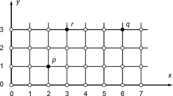
The Minkowski metrics can obviously have noninteger values, even for pairs of grid points; for example, in Figure 3.2, we have de(p,r) = ![]() . The measurements used in digital geometry are often based on integer-valued metrics.
. The measurements used in digital geometry are often based on integer-valued metrics.
We recall the definitions of the floor, ceiling, and nearest integer functions for all real a:
For any function d : S×S → R, we can define ![]() by
by ![]() (p, q) =
(p, q) =  and similarly for
 ![]() and [d]. However, even if d is a metric, these integer-valued functions may not be metrics. For example, we have the following:
and [d]. However, even if d is a metric, these integer-valued functions may not be metrics. For example, we have the following:
Proposition 3.2
![]() and [de] are not metrics on Z2.
and [de] are not metrics on Z2.
Proof Let p = (2,3), q = (−1, −1), and r = (0,0). Then ![]() ](p,q) = 5, but
](p,q) = 5, but ![]() (p,r) = 3 and
(p,r) = 3 and ![]() (r, q) = 1, so property M3 is not satisfied. For [de], use, for example, p = (1,1) and q and r as before.
(r, q) = 1, so property M3 is not satisfied. For [de], use, for example, p = (1,1) and q and r as before.
It follows that ![]() and [de] are not metrics on Rn or Zn for n ≥ 2. Interestingly,
and [de] are not metrics on Rn or Zn for n ≥ 2. Interestingly, ![]() is a metric. In fact, we have the following:
is a metric. In fact, we have the following:
Theorem 3.1
If d is a metric,![]() is also a metric.
is also a metric.
Proof Let p,q,r ∈ S, a = d(p,q), b = d(q,r), and c = d(p,r). We show that ![]() has properties M1 through M3.
has properties M1 through M3.
M1: For a ≥ 0, we have ![]() = 0 iff a = 0, such that
= 0 iff a = 0, such that  iff d(p, q) = 0 iff p = q. Furthermore, a ≥ 0 implies
 ![]() ≥ 0.
≥ 0.
M2: Because d(p,q) = d(q,p), we also have  =
= .
.
M3: We have a+b ≥ c, because d is a metric on S. First assume that a or b is an integer, for example, a = n; then  . Now assume that both a and b are not integers, so that
  and
and  . Because
  , it follows that
  .
.
In the example in Figure 3.2, we have ![]() , and
, and ![]() .
.
It is not hard to show that d is regular iff, for all distinct p, q ∈ S, there exists an r ∈ S such that d(p, r) = 1 and d(p, q) = 1+d(r, q). ![]() is a regular integer-valued metric on R2 but not on Z2. For example, let p and q be grid points that differ by 4 in one coordinate and by 3 in another coordinate. The distance (both de and
is a regular integer-valued metric on R2 but not on Z2. For example, let p and q be grid points that differ by 4 in one coordinate and by 3 in another coordinate. The distance (both de and ![]() ) between p and q is 5, but there is no r ∈ Z2 at
) between p and q is 5, but there is no r ∈ Z2 at ![]() distance 1 from p and 4 from q; such a real point would have to lie on the segment pq, but it cannot then have integer coordinates.
distance 1 from p and 4 from q; such a real point would have to lie on the segment pq, but it cannot then have integer coordinates.
Integer-valued metrics are of special interest in picture analysis. It can be shown that a finite metric space is isomorphic to the distance space on a graph (see Chapter 4) iff the metric is regular; this implies that d4 and d8 are regular. Integer-valued metrics will be discussed further in Sections 3.2 and 3.4.
3.1.5 Restricting and combining metrics
From Exercise 8 in Section 1.3, we know that [Zn,+, ·, R] is not a vector space, because it is not closed under scalar multiplication a · p (property V0). The algebraic structure [Zn,+, ·, Z] is an example of a unitary module: it satisfies properties V0 trough V8 with respect to a ring of scalars that has an additive identity.
In particular, metrics on Rn define metrics on Zn, because Zn is a subset of Rn. For example, the Minkowski metrics define metric spaces on the sets Z2 and Z3 of all 2D or 3D grid points, and they define metric spaces on rectangular grids Gm,n for all m, n (see Equation 1.1) or cuboidal grids Gl,m,n for all l,m,n, because these grids (using the grid point model) are finite subsets of Z2 or Z3.
There are ways of combining two metrics d′, d′′ on a set S so that the resulting function d is a metric on S. For example:
(i) A linear combination of two metrics, d(p, q) = a · d′(p,q)+b · d′′(p, q), where 0<a,b ∈ R is a metric.
(ii) The maximum of two metrics, d(p, q) = max{d′(p, q),d′′(p, q)}, is a metric.
On the other hand, the product or minimum of two metrics is not necessarily a metric.
3.1.6 Boundedness
The Minkowski metrics on Rn are examples of unbounded metric spaces [S, d], where S = Rn is an infinite set, and the distances between points in S can exceed any finite bound. Any metric space [S,d] on a unitary module S satisfying the homogeneity property M5 is necessarily unbounded. We now give some examples of bounded metric spaces.
We first give a degenerate example. Let S be a nonempty set, and we define that
It can easily be verified that [S, db] is a metric space, and it is evidently bounded. The function db is called the binary metric. The norm ![]() = db(p,o), defined as in Equation 3.5, satisfies N2* but not N2.
= db(p,o), defined as in Equation 3.5, satisfies N2* but not N2.
If [S, d] is an unbounded metric space,
defines a metric d′ on S, and [S, d′] is a bounded metric space.
We now give a more detailed example using the mapping that takes p = (x, y),∈ R2 into p* = (x*,y*), where the following are true:
For any p, p* is contained in a disk of radius 2. Indeed, for o = (0,0) we have the following:
(Note: c is defined in this equation.) This is true because ![]() and thus c < 1. Thus the mapping defined by Equation 3.8 is one-to-one from R2 onto the open disk of radius 2. Any (x,y) on the circle with center o and radius 4/3 is mapped into (3x/4, 3y/4), which is on the circle with center o and radius 1. Hence any point p farther than 4/3 from o is mapped into a point p* in the open annulus defined by the circles of radii 1 and 2. (The function (arctan(x), arctan(y)) is another example of a continuous one-to-one mapping from R2 into a bounded set—the open square (–π/2,π/2)2 in this case.)
and thus c < 1. Thus the mapping defined by Equation 3.8 is one-to-one from R2 onto the open disk of radius 2. Any (x,y) on the circle with center o and radius 4/3 is mapped into (3x/4, 3y/4), which is on the circle with center o and radius 1. Hence any point p farther than 4/3 from o is mapped into a point p* in the open annulus defined by the circles of radii 1 and 2. (The function (arctan(x), arctan(y)) is another example of a continuous one-to-one mapping from R2 into a bounded set—the open square (–π/2,π/2)2 in this case.)
Bounded distances between points p,q ∈ R2 can now be defined using the distances, for any metric d on R2, between p* and q* in the disk of radius 2. In other words, for any metric space [R2,d] we define the following:
If d is a metric on R2,so is d*, and d*(p, q) < 4 for all p,q ∈ R2. For example, for the integer-valued metric ![]() (see Theorem 3.1), all distances between points p, q ∈ R2 are integers in the set {0,1,2,3,4}. We sometimes have
(see Theorem 3.1), all distances between points p, q ∈ R2 are integers in the set {0,1,2,3,4}. We sometimes have ![]() note that this does not contradict the triangularity property. We can change the cardinality of the range of d* by increasing or decreasing the parameter 2 in Equation 3.8. Such metrics might be of interest for classifying pixels (pairs of integers) using finite numbers of distance values.
note that this does not contradict the triangularity property. We can change the cardinality of the range of d* by increasing or decreasing the parameter 2 in Equation 3.8. Such metrics might be of interest for classifying pixels (pairs of integers) using finite numbers of distance values.
3.1.7 The topology induced by a metric
A metric induces a topology defined by a family of open or closed sets; this section briefly addresses such issues. For a more extensive discussion of topologic subjects, see Chapter 6.
For any metric space [S, d], any p ∈ S, and any ε >0, let the following be true:
Uε(p) is called the (open)ε-neighborhood of p in S; evidently p ∈ Uε(p). The family of all ε-neighborhoods defines a basis of a topology and allows us to generate open sets by taking (finite or infinite) unions of ε-neighborhoods. The Euclidean metric de on Rn defines the Euclidean topology. For the binary metric db, we have Uε(p) = {p} for 0 <ε ≤ 1 and Uε(p) = S for ε > 1.
Definition 3.2
p ∈ S is a frontier point of A ⊆ S iff, for any ε > 0, Uε (p) contains points of A as well as points of ![]() . The frontier
. The frontier ![]() A of A consists of all frontier points of A.
A of A consists of all frontier points of A.
For example, the frontier of a disk is a circle. The interior A° of A is AvA, and the closure A• of A is A ∪ ![]() A. A is closed iff A = A• and open iff A = A °. The empty set ∅ and the set S are both closed and open.
A. A is closed iff A = A• and open iff A = A °. The empty set ∅ and the set S are both closed and open.
The interior of A is the largest open set contained in A, and the closure of A is the smallest closed set that contains A. A set is closed iff its complement is open.
A ⊆ S is bounded iff A ⊆ Uε (p) for some p ∈ S and some ε > 0. (A bounded set need not be of finite cardinality.) A is called compact iff, whenever it is contained in the union of a set of open sets, it is contained in a finite union of these sets. The Heine-Borel-Lebesgue theorem [112] says that a subset of Rn is compact in the topology defined by any Minkowski metric on R iff it is bounded and closed. A continuous real-valued function defined on a compact set always has a minimum and a maximum on that compact set.
Two metrics d and d′ on S are called topologically equivalent iff a subset of S is open with respect to d iff it is open with respect to d′. For example, the Minkowski metrics on Rn are all topologically equivalent. A bounded metric on an infinite subset of Rn (see the examples in Section 3.1.6) can be topologically equivalent to an unbounded metric. For example, the bounded metric de(p, q)/[1+de(p, q)] is topologically equivalent to the unbounded metric de; the ball of radius r in the unbounded metric corresponds to the ball of radius r/(1+r) in the bounded metric, and the ball of radius s < 1 in the bounded metric corresponds to the ball of radius s/(1 – s) in the unbounded metric.
3.1.8 Distances between sets
Any metric d on a set S can be extended to a Hausdorff metric on the family of all nonempty compact subsets A,B of S by defining

where sup and inf denote the least upper bound and greatest lower bound, respectively. (For compact sets A and B we can replace inf and sup with min and max, respectively.) Figure 3.3 shows an example of this metric in which d is the Euclidean metric de.

The definition of the Hausdorff metric can be broken up into steps. We first define the closest distance from p ∈ S to T ⊆ S using the following:
Let A, B ⊂ S; let hp(B) = d(p,B) for all p ∈ A; let hp(A) = d(p, A) for all p ∈ B; and define the following:
Then here we have the Hausdorff metric of Equation 3.9:
In Figure 3.3, we have ![]() and
and ![]() .so that d(A,B) = hA(B).
.so that d(A,B) = hA(B).
An alternative way of defining the Hausdorff metric makes use of the definition of an (open)ε-neighborhood of a set. We define that
Let hq be defined by a metric d on S;ε > 0; A ⊂ S; and ![]() be the Minkowski sum (see Section 1.2.12). Then, if A and B are nonempty compact subsets of S, we have the following:
be the Minkowski sum (see Section 1.2.12). Then, if A and B are nonempty compact subsets of S, we have the following:
Figure 3.4 illustrates this method of defining a Hausdorff distance. Uε(B) is a dilation of B; dilations will be studied in Chapter 15. Note that, for D = Uε(o), we have D = D where D is the mirror set used in the definition of dilation; see Section 1.2.12. (If A and B are compact and we dilate by a closed ball of radius ε instead of an open ball, hA(B) is defined by min instead of inf.)
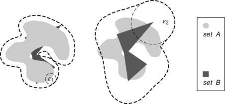
FIGURE 3.4 Left: B (a simple polygon) is completely contained in ![]() . Right: A is not completely contained in
. Right: A is not completely contained in ![]() , showing that d(A, B) > ε 2.
, showing that d(A, B) > ε 2.
The Hausdorff distance is not a metric in the family of all nonempty bounded subsets of S. For example, consider the closed unit square [0,1]2 = [0,1]×[0,1] and the open unit square (0,1)2 = (0,1)×(0,1) in the Euclidean topology of the plane.2 Then de([0,1]2, (0,1)2) = 0, but the sets are not identical, so property M1 of a metric is violated.
A generalized metric satisfies the axioms of an ordinary metric but can also have value∞. The Hausdorff distance is a generalized metric in the family of closed sets (bounded or not). We can also include the empty set; in the definition of Hausdorff distance, we replace an empty supremum with 0 and an empty infimum with∞ so that the empty set is at distance 0 from itself but at distance∞ from any nonempty set.
The Hausdorff metrics are based on maximum distances between sets; a single point (an “outlier”) in a set can strongly influence these distances. Distances between sets defined by set-theoretic differences are less sensitive to single points. The symmetric difference between two subsets A, B of a set S is as follows:
Let S be any nonempty set, and let ℘fin(S) be the family of all finite subsets of S.
Proposition 3.4
dsym and d′sym are metrics on ℘fin(S).
Proof Let A,B,C ∈ ℘fin(S), a = dsym(A,B), b = dsym(B,C), and c = dsym(A, C). We show that dsym has properties M1 through M3.
M1: a = 0 iff AΔB = ø iff A = B.
M2: Because AΔB = BΔA, we have symmetry.
M3: Let A = A1 ∪ D ∪ E ∪ F, B = B1 ∪ D ∪ E ∪ G, and C = C1 ∪ E ∪ F ∪ G (see Figure 3.5). Let a1 = card(A1), d = card(D), and so forth. It follows that a = a1+b1+f+g, b = b1+c1+d+f, and c = a1+c1+d+g. This shows that a+b = a1+2b1+c1+d+2f+g ≥ c.

For d′Sym, M1 and M2 follow by arguments similar to those for dsym. Regarding M3, let a = d′sym(A,B), b = d′sym(B,C), and c = d′sym(A,C), and consider the intersections of A, B, and C as before. Let h = b1+f+g, k = d+e+ 1, and i = a1+c1 – b1. Then the following are true:
Let a2 = a1+h, b2 = c1+h, and c2 = i+h. Because h ≥ 0 and 0 ≤ i ≤ a1+c1, we have 0 ≤ c2 ≤ a2+b2. Together with k ≥ 1, this allows us to show that a+b – c ≥ 0 so that a+b ≥ c.
dsym is the L∞ distance of the characteristic functions of sets; this provides a direct proof that it is a metric. For d′sym, we could also derive Proposition 3.4 from the more general fact that, for any metric d, the function d′ defined by d′(p,q) = d(p, q)/[1+d(p, q)] is a topologically equivalent bounded metric; note that our proof covers the general case.
3.2 Grid Point Metrics
In this section, we discuss integer-valued metrics that are related to the grid point adjacency models defined in Sections 2.1.3 and 2.1.4. We also discuss methods of defining neighborhoods and closeness; grid point metrics that approximate the Euclidean metric; paths, geodesics, and intrinsic distances; and distances between sets of grid points.
3.2.1 Basic grid point metrics
Let p,q ∈ R2, p =(x1, y1), q = (x2, y2), and define the following:
Then [R2, d4] is a metric space; in fact, d4 is the Minkowski metric L1. We call d4 the city-block metric or Manhattan metric because, when we restrict it to Z2, d4(p,q) is the minimal number of isothetic unit-length steps from p to q; it resembles a shortest walk in a city with streets that are laid out in an orthogonal grid pattern. In the example in Figure 3.2, we have d4(p,r) = 3, d4(p, q) = 6, and d4(r, q) = 3.
Let p,q ∈ R2,p =(x1, y1), and q = (x2, y2), and define the following:
Then [R2,d8] is a metric space; in fact, d8 is the Minkowski metric L∞. Thus d8 is called the chessboard metric because, when we restrict it to Z2, d8(p, q) is the minimal number of moves from p to q by a king on a chessboard. In the example in Figure 3.2, we have d8(p,r)= 2, d8(p,q) = 4, and d8(r,q) = 3.
Let S ⊆ R2, let o = (0,0) ∈ S, and let d be a metric on S. The set {p : p ∈ S Λ d(p, o) ≤ 1} is called a unit disk in [S, d]. Figure 3.6 shows the unit disks in R2 for the metrics d4, de, and d8.

For any grid point p, the smallest neighborhood of p in [Z2, da] (α ∈ {4,8}) is defined by the following:
The notations d4 and d8 are suggested by the fact that N4(p) – {p} has cardinality 4 and N8(p) – {p} has cardinality 8. Using Equation 3.4, we have the following:
The last inequality is an easy consequence of the definitions of d8 and d4: without loss of generality, let d8(p,q) = ![]() then d4(p,q) ≤ 2 ·
then d4(p,q) ≤ 2 · ![]() = 2·d8(p,q).
= 2·d8(p,q).
Let p,q ∈ R3, p =(x1, y1, z1), and q = (x2, y2, z2), and define the following:
(This definition is equivalent to the one based on 18-paths; see Theorem 3.6.) For any grid point p, the smallest neighborhood of p in [Z3, dα] (α ∈ {6, 18, 26}) is defined by the following:
Note that Nα(p) – {p} has cardinality α for α = 6, 18, and 26. Analogous to Theorem 3.2 and using Equation 3.4, we have the following (see also Exercise 3 in Section 3.5):
Theorem 3.3
d26(p,q) ≤ de(p,q) ≤ d6(p,q) ≤ 3 · d26(p,q) for all p,q ∈ R3, and d26(p,q) ≤ d18(p,q) ≤ de (p,q) for al1 p,q ∈ Z3 such that de (p,q) ≠ ![]() .
.
Proof d26(p,q) ≤ d18(p,q) follows from the definition of d18. For d18(p,q) ≤ de(p,q), we need only to show that ![]() ≤ de(p,q), because L∞(p,q) = d26(p,q) ≤ de(p,q) = L2(p,q).
≤ de(p,q), because L∞(p,q) = d26(p,q) ≤ de(p,q) = L2(p,q).
If 0 (p,q) < 1, then ![]() = 1 and
= 1 and ![]() > d6 (p,q) ≥ de(p,q). If p,q ∈ Z3 and d6 (p, q) = 0 or d6 (p, q) = 1, we have
> d6 (p,q) ≥ de(p,q). If p,q ∈ Z3 and d6 (p, q) = 0 or d6 (p, q) = 1, we have ![]() = d6(p, q) = de(p, q).
= d6(p, q) = de(p, q).
If 1 < d6(p, q), then ![]() < d6(p, q). If p,q ∈ Z3 and d6(p, q) = 2, we have de(p,q) = 2 or de(p,q) =
< d6(p, q). If p,q ∈ Z3 and d6(p, q) = 2, we have de(p,q) = 2 or de(p,q) =![]() , such that
, such that ![]() = 1 < de(p,q). If p,q ∈ Z3 and d6(p, q) = 3, we have de(p, q) = 3, de(p, q) =
= 1 < de(p,q). If p,q ∈ Z3 and d6(p, q) = 3, we have de(p, q) = 3, de(p, q) = ![]() , or de(p, q) =
, or de(p, q) = ![]() , such that
, such that ![]() = 2 > de(p, q) in the latter case. However, if p,q ∈ Z3 and d6(p, q) ≥ 4, then
= 2 > de(p, q) in the latter case. However, if p,q ∈ Z3 and d6(p, q) ≥ 4, then ![]() ≤ de(p, q).
≤ de(p, q).
3.2.2 Neighborhoods and degrees of closeness
The ε-neighborhood Uε(p) (see Section 3.1.7) is defined for any metric space [S,d], any p ∈ S, and any ε > 0. In some cases we have Uε(p) = {p}; for example, this is true for ε ≤ 1 and any of the metrics [de], d4, and d8 on Z2 or for the binary metric.
If the range of d is countable so that Uε is of interest only for discrete values of ε (e.g., for metrics on a grid G that is a subset of Z2, Z3, Z2,or Z3), we use the notation e-neighborhood instead of ε-neighborhood. The e-neighborhoods for three metrics on ![]() are illustrated in Figure 3.7; see Figure 3.6 for the corresponding disks in the real plane. The metrics d4, de, and d8 are translation-invariant; hence the sets Uε(p) have identical “shapes” for all p.
are illustrated in Figure 3.7; see Figure 3.6 for the corresponding disks in the real plane. The metrics d4, de, and d8 are translation-invariant; hence the sets Uε(p) have identical “shapes” for all p.

FIGURE 3.7 The e-neighborhoods for e = 1,2,3,4, and 5 in the 2D grid cell model defined by the city block (left), Euclidean (middle), and chessboard (right) metrics.
For any metric d on a grid G, there is an interval of values e >0 such that Ue(p) contains as few grid points as possible in addition to p itself. This minimal set of grid points is called the smallest (nontrivial) neighborhood N(p) of p with respect to d. (In the grid cell model, we use the notationη(β), where c is a cell.) For example, for dα (α ∈ {4,6,8,18,26}), the smallest neighborhoods Nα(p) defined in Section 3.2.1 are obtained for 1 < e ≤ 2. For e = 1, we have U1(p) = {q ∈ Z2 : dα(q,p) <1} = {p} for any of these dαs.
With fuzzy geometry (see Section 1.2.10), we can define the degree of closeness of two points p and q of a metric space [S, d] as a monotonically nonincreasing function of the distance between p and q. For example, we can define c(p, q) = 1/[1+d(p, q)]. It follows that 0 <c(p, q) ≤ 1 for all p, q; hence, for any p, c(p, q) defines a fuzzy subsetμρ of S{p} that we can think of as a fuzzy neighborhood of p.
Degrees of closeness between pixels or voxels p and q in a picture P can be defined using monotonically nonincreasing functions of the absolute difference between P(p) and P(q). For example, we can define c′(p,q) = 1/(|P(p) – P(q)|+ 1). Note that, for any p and q, we have 1/(Gmax+ 1) ≤ c′(p,q) ≤ 1 so that c′(p,q) defines a fuzzy subsetμ′ρ of the picture. We can also define degrees of closeness between pixels or voxels that depend on both the distance between them and the absolute difference between their values. In Section 3.4, we will define a metric on a picture in which the distance from p to q depends on the sums of the pixel or voxel values along paths from p to q.
3.2.3 Approximations to the Euclidean metric
We saw in Figure 3.6 that the set of points within a given d4 or d8 distance from a given point is a square. These distances depend on direction; their “disks” are not good approximations to Euclidean disks. If we restrict d4 and d8 to Z2 the set of grid points q such that d4(p, q) ≤ k is a diagonally oriented square (a “diamond”) of odd diagonal length 2k + 1 centered at p, and the set of grid points q such that d8(p,q) ≤ k is an upright square of odd side length 2k + 1 centered at p; see Figure 3.7.
Better approximations to Euclidean disks can be obtained by combining d4 and d8, for example, by taking the following:
It is not hard to see that the set of grid points such that d(p, q) ≤ k is the intersection of an upright square of side length k with a diamond of diagonal length 3k/2; this intersection is an upright octagon. Varying the coefficient of d4 in Equation 3.11 causes the shape of the octagon to vary between a diamond and a square. The octagon can be made arbitrarily close to regular by choosing the coefficient appropriately.
Metrics with disks that are “hexagons” can be defined by using a modification of the standard orthogonal grid in which, for example, the odd-numbered rows are shifted half a unit to the right; see Figure 3.8. This is equivalent to working with an unshifted grid but treating a grid point) on an odd-numbered row as having the six neighbors (i ± 1,j), (i,j ± 1), and (i+1, j ± 1) and a grid point on an even-numbered row as having the six neighbors (i ± 1, j), (i,j ± 1), and (i − 1, j ± 1).
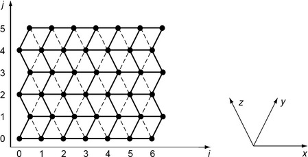
FIGURE 3.8 Modification of the standard grid in which the odd-numbered rows are shifted half a unit to the right.
In the hexagonal grid shown in Figure 3.8, we can introduce a coordinate system by using any two of the three axes shown on the right, for example, x and y. We can
reach any grid point p from the origin by making an (positive, negative, or zero) integer number u of moves in the+ x direction and then an integer number v of moves in the+ y direction; the resulting (u,v) are the coordinates of p. We will use these coordinates in the remainder of this discussion.
The x,y, and z axes divide the plane into six sextants that we number counterclockwise beginning at the+ x axis; see the figure in Exercise 2 in Section 1.3. It is easily verified that the signs of the (u, v) coordinates of the points lying in these sextants can be characterized as shown in Table 3.1. Note that the z-axis is the locus of points such that u+v = 0.

The hexagonal distance between two points p and q of the hexagonal grid is the minimum number of unit moves in the x and y directions needed to go from p to q. If p = (i,j) and q =(h, k), it can be shown that this number is given as follows:
(The signum function sgn(a) is 1 if a ≥ 0 and 0 otherwise.)
It can be shown that dh((i,j), (h, k)) is also equal to the following:
It can also be shown that hexagonal coordinates (u, v) are related to Cartesian coordinates (i,j) by the following for j even:
and by the following for j odd:
Obviously, ![]() is the integer-valued metric that best approximates de. However, “incremental” algorithms for distance computation on a grid (see Section 3.4) normally use local neighborhoods; this makes it easy to compute metrics such as d4, dh,or d8 or octagonal metrics, but not
is the integer-valued metric that best approximates de. However, “incremental” algorithms for distance computation on a grid (see Section 3.4) normally use local neighborhoods; this makes it easy to compute metrics such as d4, dh,or d8 or octagonal metrics, but not ![]() . For a method of computing a good approximation to de, see Section 3.4.3.
. For a method of computing a good approximation to de, see Section 3.4.3.
We conclude this section by describing a general method of defining approximations to Euclidean distance by counting moves in different directions (e.g., isothetic moves, diagonal moves). Let p,q ∈ Z2, and letρ be a sequence of king’s moves from p to q. Let la,b (p) = ma+nb where m is the number of isothetic moves and n the number of diagonal moves, and let the following be true:
Thus da,b is called the (a, b) chamfer distance (or weighted distance) from p to q. Chamfer distances that closely approximate Euclidean distance can be defined by appropriately choosing a and b. If the following is true,
the (a, b) chamfer distance da,b is a metric [738], which also defines a norm ![]() = da,b(p, o) (the distance of p from the origin o = (0,0)). This metric is a nonnegative linear combination of d4 and d8. Convex linear combinations of d4 and d8 also give useful chamfer distances; for example, (d4+2d8)/3 is the (3,4) chamfer distance (see Exercise 12 in Section 3.5).
= da,b(p, o) (the distance of p from the origin o = (0,0)). This metric is a nonnegative linear combination of d4 and d8. Convex linear combinations of d4 and d8 also give useful chamfer distances; for example, (d4+2d8)/3 is the (3,4) chamfer distance (see Exercise 12 in Section 3.5).
[761] formulated necessary and sufficient conditions for a 2D chamfer distance d to define a norm ![]() = d(p, o) on Z2.
= d(p, o) on Z2.
We can similarly define 3D chamfer distances da,b,c where a, b, and c correspond to moves in which only one coordinate changes (isothetic moves), two coordinates change, and all three coordinates change, and we can obtain good approximations to Euclidean distance by appropriately choosing a, b, and c.
Generalized chamfer distances can be defined using additional types of moves that are not necessarily moves between 8-neighbors or 26-neighbors.
3.2.4 Paths, geodesics, and intrinsic distances
A sequence ρ of grid points (p0, p1,…, pn) such that p0 = p, pn = q, and pi+1 is α-adjacent to pi (0 ≤ i ≤ n −1) is called an α-path of length n from p to q; p and q are called the endpoints ofρ.
An α-path is called an α-geodesic if no shorter α-path with the same endpoints exists.
Theorem 3.4
The length of a shortest α-path from p to q is dα(p, q).
Proof We give the proof in 2D for α = 4; the proofs for other cases are similar. If the length of the path is 1 (e.g., the path is (p, q)), p and q are 4-adjacent, so d4(p,q) = 1. We proceed by induction on the shortest length. Let (p0, p1,…, pn) be a shortest 4-path; then, using Proposition 3.7, (p0, p1,…, pn−1) is a shortest path from p to pn−1, so d4(p,pn−1) = n−1 by the induction hypothesis. Because q is 4-adjacent to pn−1, we have d4(pn−1, q) = 1 so that, by the triangle inequality, d4(p,q) ≤ (n−1) +1 = n. If d4(p, q) = m <n, we can easily construct a 4-path of length m from p to q. For example, suppose p =(i,j) and q = (h,k) where i ≤ h and j ≤ k; the argument is similar if i ≥ h and/or j ≥ k. Because d4(p, q) = m, we have (h − 1)+(h – j) = m, and we can construct a 4-path from (i,j) to (h,k) by first increasing i by 1 until it reaches h and then increasing j by 1 until it reaches k; this 4-path has length ![]() = m <n, which is contrary to our assumption that a shortest 4-path from (i, h) to (j, k) has length n.
= m <n, which is contrary to our assumption that a shortest 4-path from (i, h) to (j, k) has length n.
It follows that an α-path ρ of length n is an α-geodesic iff the dα-distance between the endpoints ofρ is n.
In Euclidean space, there is a unique shortest arc between any two points p and q, which is namely the straight line segment pq. In a grid, there can be many shortest α-paths between two grid points, and these paths need not be digital straight line segments (see Section 2.3.4 and Chapter 9). In what follows, we consider only the 2D cases α = 4 and 8, and we assume that pi (0 ≤ i ≤ n) has coordinates (xi, yi).
Proposition 3.8
The following properties of a 4-path ρ are equivalent:
(b)ρ cannot turn right (or left) twice in succession; left and right turns must alternate.
(c) x0 ≤ x1 ≤… ≤ xn (or all ≥), and y0 ≤ y1 ≤… ≤ yn (or all ≥).
Proof To see that (a) implies (b), suppose thatρ made two successive turns in the same direction:

(The argument in other cases is analogous.) Then the subpath ofρ from pr to ps has length s – r, but there is a horizontal path from pr to ps of length s – r − 2, so Proposition 3.7 is violated, andρ cannot be a 4-geodesic.
We next show that (b) implies (c). Suppose the initial direction ofρ is horizontal toward the right and its first turn (if any) is a left turn; the proofs in other cases are analogous. Let the turns be at pn1, pn2 where 0 <n1 <n2 <… <n; then x0 <x1 <… <xn1, and y0 = y1 = … = yn1. After the first turn,ρ is headed vertically upward; thus xn1 = xn+1 = …. = xn2, and yn1 <yn+1 <… <yn2. By (b), the second turn must be a right turn, after whichρ is again horizontal and headed rightward, so xn2+1 <… <xn3, yn+1 = … = yn3, and so on, proving (c). Note that, by (c), if we take any pm onρ as origin, the subpaths (p0,…, pm) and (pm,…, pn) must lie in a pair of opposite quadrants.
Next we prove that (c) implies (d). At each step along a 4-path, either x or y (but not both) changes by 1. Hence, if (c) holds (e.g., x0 ≤ x1 ≤ … ≤ xn and y0 ≤ y1 ≤ …. ≤ yn and similarly in the other cases), the number of steps at which the xs increase and the number at which the ys increase must add up to n, which implies (d).
Finally we show that (d) implies (a). Any 4-path from (x0, y0) to (xn, yn) must have length at least ![]() , because a coordinate can change by only 1 at each step, and only one coordinate can change at a time. If (d) holds, this length is n, and becauseρ has length n, its length is the shortest possible, thus proving (a).
, because a coordinate can change by only 1 at each step, and only one coordinate can change at a time. If (d) holds, this length is n, and becauseρ has length n, its length is the shortest possible, thus proving (a).
These results imply that digital straight line segments (see Chapter 9) are geodesics. It is not hard to show that the only possible turns in an 8-geodesic are 45° right and left turns in alternation.
If S is an α-connected set of grid points (see Chapter 4), for any p,q ∈ S, there exists an α-pathρ =(p0, p1,…, pn) from p0 = p to pn = q such that the pis are all in S. The length ![]() of a shortest such path is called the intrinsic α-distance in S from p to q. The ordinary α-distance from p to q will sometimes be called extrinsic to contrast it with intrinsic α-distance.3
of a shortest such path is called the intrinsic α-distance in S from p to q. The ordinary α-distance from p to q will sometimes be called extrinsic to contrast it with intrinsic α-distance.3
Proposition 3.10
dα(p,q) ≤ ![]() (p,q) for all p,q ∈ S.
(p,q) for all p,q ∈ S.
Proof The length of a shortest α-path that lies in S cannot be less than the length of an unrestricted shortest α-path. ∈
We will see in Chapter 13 that a set S of grid points is digitally convex iff any two points of S are the endpoints of a digital straight line segment that is contained in S. Because a digital straight line segment is a geodesic, it follows that, if S is digitally convex, ![]() , (p,q) is equal to dα(p,q) for all p,q ∈ S.
, (p,q) is equal to dα(p,q) for all p,q ∈ S.
3.2.5 Distances between sets
Integer-valued metrics d on a grid, such as ![]() , d4, and d8 in 2D, define Hausdorff metrics in the family of all finite subsets of the grid; see Section 3.1.8 For any such d, any grid point p, and any finite set of grid points S, the distance from p to S is hp(S) = min d(p,q) where the min is taken over all q ∈ S. Evidently, hp(S)= 0 iff p ∈ S. For example, for the p, q, and r in Figure 3.2, let A = {p, q} and B = {q,r}; then d4 (A, B)= d4(p,r) = d4(r,q) = 3, d8(A, B) = d8(p,r)= 2, and
, d4, and d8 in 2D, define Hausdorff metrics in the family of all finite subsets of the grid; see Section 3.1.8 For any such d, any grid point p, and any finite set of grid points S, the distance from p to S is hp(S) = min d(p,q) where the min is taken over all q ∈ S. Evidently, hp(S)= 0 iff p ∈ S. For example, for the p, q, and r in Figure 3.2, let A = {p, q} and B = {q,r}; then d4 (A, B)= d4(p,r) = d4(r,q) = 3, d8(A, B) = d8(p,r)= 2, and ![]() (A,B) =
(A,B) = ![]() (p,r) =
(p,r) = ![]() (r,q) = 3. Similarly, for the sets A and B in Figure 3.3, we have d4(A,B) = hp(B) = 8 > hq(A) = 6(hp and hq with respect to d4) and d8(A,B) = hp(B)=hq(A)= 5(hp and hq with respect to d8).
(r,q) = 3. Similarly, for the sets A and B in Figure 3.3, we have d4(A,B) = hp(B) = 8 > hq(A) = 6(hp and hq with respect to d4) and d8(A,B) = hp(B)=hq(A)= 5(hp and hq with respect to d8).
A Hausdorff metric can be used to measure the distance between the frontiers of the inner and outer Jordan digitizations of a set; see Figure 2.29 for an example. Section 3.1.7 allows us to complete Definition 2.8: the inner Jordan digitization ![]() (S)
(S)
of a set S ⊆ Rn is actually the union of all n-cells (for grid resolution h > 0 and n = 2 or n = 3) that are contained in the interior of set S.
Theorem 3.5
For any compact set S ⊂ R2 such that ![]() (S) ≠ ø, the d4 or d8 Hausdorff distance between the (polygonal) frontiers
(S) ≠ ø, the d4 or d8 Hausdorff distance between the (polygonal) frontiers ![]() (S) and
(S) and ![]() (S) is at least 1/h
(S) is at least 1/h
Proof Let p be an arbitrary grid vertex on ![]() (S). Thus p cannot be on
(S). Thus p cannot be on ![]() (S), because the frontier of
(S), because the frontier of ![]() (S) never intersects the frontier of
(S) never intersects the frontier of ![]() (S) if S is a nonempty compact subset of R2. The d4 (or d8) distance from p to any point q on
(S) if S is a nonempty compact subset of R2. The d4 (or d8) distance from p to any point q on ![]() (S) is at most 1/h. It follows that
(S) is at most 1/h. It follows that
Finally, we discuss algorithms for calculating the Hausdorff distance between two finite sets A,B ⊂ Gm,n of grid points (see Algorithm 3.1). We assume that m and n are the dimensions of the smallest isothetic rectangle that contains A ∪ B.
We first describe a brute-force approach. For every point in A, calculate the minimum distance to a point in B, and, for every point in B, calculate the minimum distance to a point in A. Take the maxima of these two sets of distances; then the maximum of the two maxima is the desired Hausdorff distance. The points of A and B can be located by scans of Gm,n (see Section 1.1.3); on one scan, we find all of the points p in A, and, for each p, we scan Gm,n again to find all of the points in B and calculate the distances from p to these points. If card(A) and card(B) are O(mn), this brute-force algorithm takes O(m2n2) computation steps.
A much more efficient algorithm is shown above. For any S ⊂ Gm,n, the distance field F (S) is an array of size m×n such that F (S)(p) = hp (S); in particular, F (S)(p)= 0 iff p ∈ S. It can be shown (see Section 3.4.2 for grid metrics and Section 3.4.3 for the Euclidean metric) that F (S) can be calculated in O(mn) computation steps for any Minkowski metric on Gm,n. This allows us to calculate the Hausdorff distance in O(mn) computation steps by computing distance fields for A and B and scanning each of these fields.
3.3 Grid Cell Metrics
In Sections 3.1.2 and 3.1.3, we defined metric-related concepts such as norms, scalar products, and angular values in n-dimensional vector spaces. In this section, we apply these concepts to the n-dimensional unitary modules defined by the grid cell model. Results involving grid cell adjacency models easily translate into results involving the isomorphic grid point adjacency models.
3.3.1 Basic grid cell metrics
We first consider the 2D grid cell model. Let d be a metric defined on the set Z2 of grid points. For any two 2-cells c1,c2∈ ![]() , we define∂(c1, c2) by the value of d for the center points of c1 and c2;∂ is thus a metric on
, we define∂(c1, c2) by the value of d for the center points of c1 and c2;∂ is thus a metric on ![]() . When d = d4, we call this metric∂1, and, when d = d8, we call it∂0. Evidently,∂1(c1, c2) ≤ 1 iff c1 ∩ c2 contains (at least) one 1-cell, and∂0(c1, c2) ≤ 1 iff c1 ∩ c2 contains (at least) one 0-cell; the subscript indicates the dimension of the cells that have to be contained in the intersection. Smallest neighborhoods in the grid cell model are denoted by the following:
. When d = d4, we call this metric∂1, and, when d = d8, we call it∂0. Evidently,∂1(c1, c2) ≤ 1 iff c1 ∩ c2 contains (at least) one 1-cell, and∂0(c1, c2) ≤ 1 iff c1 ∩ c2 contains (at least) one 0-cell; the subscript indicates the dimension of the cells that have to be contained in the intersection. Smallest neighborhoods in the grid cell model are denoted by the following:
The 2D (grid cell) incidence model also includes 1-cells and 0-cells; it was illustrated in Figure 2.3, and in a more abstract way in Figure 2.13. The set of centers of the 2-, 1-, and 0-cells in ![]() 2 is the grid with grid constant θ= 0.5. For any metric d on this grid and any b,c ∈
2 is the grid with grid constant θ= 0.5. For any metric d on this grid and any b,c ∈ ![]() 2,∂(b, c) is defined by the value of d for the center points of b and c; thus d is a metric on
2,∂(b, c) is defined by the value of d for the center points of b and c; thus d is a metric on ![]() 2. For example (see Figure 2.3), the 2-cell with its center at (1,2) and the 0-cell at (15,45) are at Euclidean distance
2. For example (see Figure 2.3), the 2-cell with its center at (1,2) and the 0-cell at (15,45) are at Euclidean distance ![]() , city block distance 3, and chessboard distance 5/2.
, city block distance 3, and chessboard distance 5/2.
Metrics on ![]() or
or ![]() 3 can be defined as they were in the 2D case by identifying cells with their centers. For any two 3-cells c1, c2∈
3 can be defined as they were in the 2D case by identifying cells with their centers. For any two 3-cells c1, c2∈ ![]() ,∂(c1, c2) is defined by the value of a grid point metric d for the center points of c1 and c2; thus∂ is a metric on
,∂(c1, c2) is defined by the value of a grid point metric d for the center points of c1 and c2; thus∂ is a metric on ![]() . The metrics defined in this way by d6, d18, and d26 will be denoted by∂2, ∂1, and∂0, respectively. Evidently,∂2(c1, c2) ≤ 1 iff c1 ∩ c2 contains (at least) one
. The metrics defined in this way by d6, d18, and d26 will be denoted by∂2, ∂1, and∂0, respectively. Evidently,∂2(c1, c2) ≤ 1 iff c1 ∩ c2 contains (at least) one
2-cell,∂1(c1, c2) ≤ 1 iff c1 ∩ c2 contains (at least) one 1-cell, and∂0(c1, c2) ≤ 1 iff c1 ∩ c2 contains (at least) one 0-cell. The smallest neighborhoods are as follows:
Figure 3.9 shows the (smallest) neighborhoods of 3-cells at d6-, d18-, and d26-distance ≤ 1 from a given 3-cell; they are “balls” of 3-cells of radius 1. A general definition of such metrics will be given in Section 3.3.2 for the n-dimensional grid cell model ![]() .
.

3.3.2 Seminorms
An n-cell (n ≥ 2) is an n-dimensional grid (hyper)cube with edges of length 1 with its center at a grid point p ∈ Zn. [![]() ,+, ·, Z] is a unitary module. We identify cells by their centers; hence, if p is the center of n-cell c ∈
,+, ·, Z] is a unitary module. We identify cells by their centers; hence, if p is the center of n-cell c ∈ ![]() , k ·c is the n-cell with its center at k · p, and –c is the n-cell with its center at –p.
, k ·c is the n-cell with its center at k · p, and –c is the n-cell with its center at –p.
Let the following be true (0 ≤ i <n):
Bi is a subset of the frontier of the n-dimensional cube [−1,+ 1]n. For example, B0 = {−1,+ 1}n is the set of all vertices of this cube. We always have o = (0,…,0) ∉ Bi. Because i <n, we have xk ≠ 0 for at least one coordinate k.
Let c∈ ![]() be an n-cell, let 0 ≤α <n, and let
be an n-cell, let 0 ≤α <n, and let
where ![]() is the Minkowski sum defined in Section 1.2.12 Then the following is true:
is the Minkowski sum defined in Section 1.2.12 Then the following is true:
For example, for n = 3, we have card (η0(c)) = 27. Two n-cells c1 and c2 are called α-neighbors iff c1 ∈ ηα(c2). This defines the n-dimensional grid cell adjacency models.
Let the following be true for 0 ≤α <n and t ≥ 0:
Let ![]() be the smallest t such that c ∈
be the smallest t such that c ∈ ![]() , where c ∈
, where c ∈ ![]() . Here,
. Here, ![]() is called the α-value of c. For example, for n = 2, we have c0 = max{|x|, |y|} and ci = |x|+|y| where x and y are the coordinates of the center of c.
is called the α-value of c. For example, for n = 2, we have c0 = max{|x|, |y|} and ci = |x|+|y| where x and y are the coordinates of the center of c.
Theorem 3.6
Let c ∈ ![]() ,c =(x1,…, xn), and 0 ≤α <n. Then the following is true:
,c =(x1,…, xn), and 0 ≤α <n. Then the following is true:
Proof By induction on t, it can be shown that the following is true:

For α = 0 and α = n−1, we obtain the following norms:
This coincides with the Minkowski norm ![]() ; see Section 3.1.2 We also obtain the following:
; see Section 3.1.2 We also obtain the following:
This coincides with the Minkowski norm ![]() . For 1 ≤α ≤ n − 2, k = n – α, and c =(k − 1, k, …, k), we have cα = n (recall that n ≥ 2), and thus we have the following:
. For 1 ≤α ≤ n − 2, k = n – α, and c =(k − 1, k, …, k), we have cα = n (recall that n ≥ 2), and thus we have the following:
Thus, for 1 ≤α ≤ n − 2, the α-value ·α is not a norm but rather a seminorm, which also satisfies –cα = cα for all c ∈ ![]() and all 0 ≤α <n. As in Equation 3.3, we define the following for all c1, c2∈
and all 0 ≤α <n. As in Equation 3.3, we define the following for all c1, c2∈ ![]() :
:
For example, for n = 3 and α = 1,∂1 is identical to the metric d18 defined in Section 3.2.1
Theorem 3.7
∂a (0 ≤α <α) is a regular metric on ![]()
Proof An α-path of length m − 1 from c1 to cm ≠ c1 is a sequence of n-cells (c1, c2,…, cm−1, cm) such that ci is an α-neighbor of ci+1 and ci ≠ ci+1 (1 ≤ i ≤ m − 1). First, we show that cα is equal to the length of an α-geodesic (c1, c2,…, cm) from the origin o to c = cm. Let bi+1 = ci+1 – ci (1 ≤ i ≤ m − 1).
and let c = b2+b3+ …+bm so that c ∈ ![]() and cα ≤ m − 1. On the other hand, for any c ∈
and cα ≤ m − 1. On the other hand, for any c ∈ ![]() , there exists an α-path of length m − 1 from o to c so that the length of an α-geodesic from o to c is at most cα.
, there exists an α-path of length m − 1 from o to c so that the length of an α-geodesic from o to c is at most cα.
We have shown that, for any c1 ≠ c2,∂α(c1, c2)= c2 – c1 = m − 1 ≥ 1 is the length of an α-geodesic from c1 to c2. Let (b1,b2,…, bm) be an α-geodesic from b1 = o to bm = c2 – c1; then (b1+c1, b2+c1,…, bm+c1) is an α-geodesic from c1 to c2. Let c3 = b2+c1; then∂α(c1, c3) = 1 and∂α(c1, c2) = 1+∂α(c3, c2), because (b2+c1,…, bm+c1) is an α-geodesic from c3 to c2. ∈
Theorem 3.6 shows that the metrics∂α satisfy the following:
This complements Theorems 3.2 and 3.3.
3.3.3 Scalar products and angles
The seminorms || · || α define weak scalar products 〈 ·, · 〉 α (see Section 3.1.3), which satisfy the generalized Schwarz inequality on Zn. It follows that they define angular values Hα(c1, c2, c3) (see Equation 3.7). Following Proposition 3.1, Hα(c1, c2, c3) is always in the range of the arccos function.
Angular values can be used to characterize 3-cell configurations. We say that c2 is between c1 and c3 according to the α-metric (notation: (c1, c2, c3)α) iff || c1 – c3 || α = || c1 – c2 || α + || c2 – c3 || α. We call c1, c2, and c3α-cogeodetic iff they are contained in an α-geodesic; this is equivalent to (c1, c2, c3)α, (c1, c3, c2)α,or (c2, c1, c3)α
Some values of H0 and H1 for n = 2 are given in Tables 3.2 and 3.3. In both tables, o =(0,0) and c =(13,8) are fixed 2-cells, and the values H0(o,b,c) or H1(o,b,c) are given by the positions of the variable 2-cell b. From these examples, it is clear that (c1, c2, c3)α does not imply Hα(c1, c2, c3) = −1. H1(o,b,c)= 0 indicates a position for which o – b = ![]() and c – b =
and c – b = ![]() are orthogonal with respect to metric∂α.
are orthogonal with respect to metric∂α.


We saw in Section 3.3.2 that, if α = 0 or α = n−1, ·α is a norm. Hence we always have 〈 c,c 〉 0 = c20 and 〈 c,c 〉 n−1 = c2n−1, but, for 1 ≤α ≤ n−2, there exist n-cells c such that 〈 c,c 〉 α <c2α. Because 〈 b,c〈 α = −〈 b, –c 〉 α and –cα = cα for
all b,c ∈ ![]() (0 ≤α <n), the angular values are symmetric, as we see in Tables 3.2 and 3.3.
(0 ≤α <n), the angular values are symmetric, as we see in Tables 3.2 and 3.3.
The weak scalar products 〈 ·, ·)α are not homogeneous; for any α (0 ≤α <n), there exist pairs of cells b1 and b2 and c1 and c2 such that 2· 〈 b1, b2〈 α <〈 2b1, b2 〉 α and 2 · 〈 c1, c2 〉 α > 〈 2c1, c2 〉 α. It follows that these products are not linear.
3.4 Metrics on Pictures
Let P be a picture with pixel or voxel values that have been divided by Gmax so that they are in the range [0,1]. Let p and q be pixels or voxels of P, and letρ =(p0,…, pn) be an α-path from p = p0 to q = pn. We define the value-weighted length ofρ as follows:
We define the value-weighted distance dP (p,q) as minplP (ρ) where the min is taken over all α-pathsρ from p to q.
Because the reversal of a path from p to q is a path from q to p and the concatenation of a path from p to q with a path from q to r is a path from p to r, dP is symmetric and satisfies the triangle inequality, and evidently it is nonnegative. However, dP is not positive definite (metric property M1); for example, if p and q are α-adjacent and P(p) = P(q) = 0, we have dP(p,q) = 0 even though p ≠ q. On the other hand, if P(p) ≠ 0, we have dp(p, q) ≠ 0 for any q ≠ p, because any α-path from p to q must go from p to some p′ ≠ p, and the pair (p,p′) contributes a nonzero quantity ½ (P (p) + P (p′)) to the sum. Thus dP is a metric if we restrict it to the set of pixels or voxels with values that are nonzero or even if we restrict it to pairs (p, q) with values that are not both zero. (The latter is not a restriction of dP to a set of pixels or voxels, but it justifies our studying the [value–weighted] distance from non-0s to 0s in the next section.)
When we restrict dP to 〈 P 〉 (the set of pixels or voxels with values that are 1), we evidently have lP(ρ)= n and dP(p,q) = dα(p,q) for all p,q ∈ 〈 P 〉. In the next sections, we will study 4- and 8-distances from the pixels of 〈 P 〉 to the subset 〈 P 〉 in a 2D binary picture.
3.4.2 Distance transforms
Let P be a binary picture in which ![]() and
and ![]() are proper subsets of the grid. For any grid metric dα, the dα distance transform of P associates with every pixel p of 〈 P 〉, the dα distance from p to
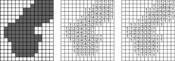
are proper subsets of the grid. For any grid metric dα, the dα distance transform of P associates with every pixel p of 〈 P 〉, the dα distance from p to ![]() .4 The dα distance transform of the set of gray pixels in the picture shown on the left in Figure 3.10 is shown for α = 4 in the middle and for α = 8 on the right.
.4 The dα distance transform of the set of gray pixels in the picture shown on the left in Figure 3.10 is shown for α = 4 in the middle and for α = 8 on the right.
We will assume in the rest of this section that the pixels outside of a rectangular region G all have value 0. We will now show that the d4 or d8 distance transform of P can be computed by performing a series of local operations while scanning G twice. (A local operation gives each pixel p a new value that depends only on the old values of the neighbors of p.)
For any p ∈ G, let B(p) (“before”) be the set of pixels (4- or 8-) adjacent to p that precede p when G is scanned row by row from top to bottom when each row is scanned from left to right (see Section 1.1.3); thus, if p has coordinates (x,y), B contains (x,y + 1) and (x − 1, y), and if we use 8-adjacency, it also contains (x − 1, y + 1) and (x+1, y+ 1). Let A(p) (“after”) be the remaining (4- or 8-) neighbors of p.
We can compute f1 (p) for every pixel in G in a single left-to-right, top-to-bottom scan of G, because for each p, f1 has already been computed for all of the qs in B(p). (If p is on the top row or in the left column of G, some of these qs are outside G, but we know that f1 = 0 for these qs because they are in ![]() .)
.)
Now let the following be true:
We can compute f2 (p) for every pixel in G in a single right-to-left, bottom-to-top scan of G, because for each p, f2 has already been computed for all of the qs in A(p) or is known because they are outside of G.
The f1s that use 4- and 8-adjacency are shown in Figure 3.11 for the picture on the left in Figure 3.10. The f2s are not shown in Figure 3.11, because they are the same as the d4s (d8s) shown in Figure 3.10, as we see from the following:
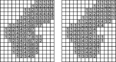
FIGURE 3.11 The first stage in computing the distance transform of the binary picture on the left in Figure 3.10. Left: d4 transform. Right: d8 transform.
Theorem 3.8
f2(p) = d(p, ![]() ) for all p ∈ G where d = d4 for the 4-adjacency version of the algorithm and d= d8 for the 8-adjacency version.
) for all p ∈ G where d = d4 for the 4-adjacency version of the algorithm and d= d8 for the 8-adjacency version.
Proof Evidently, if f2(p) = 0, p must be in ![]() . Suppose f2(p) = d(p, 〈 P 〉) for all p such that f2(p) <n, and let f2(p)=n gt;0. Then either some q ∈ A(p) has f2(q)=n − 1 or else f1(p)=n, which implies that some q ∈ B(p) has f1(q) = n − 1. In either case, using the induction hypothesis, d(q,
. Suppose f2(p) = d(p, 〈 P 〉) for all p such that f2(p) <n, and let f2(p)=n gt;0. Then either some q ∈ A(p) has f2(q)=n − 1 or else f1(p)=n, which implies that some q ∈ B(p) has f1(q) = n − 1. In either case, using the induction hypothesis, d(q, ![]() )= n − 1 so that d(p,
)= n − 1 so that d(p, ![]() ) <n. If d(p,
) <n. If d(p, ![]() ) <n, we must have d(q,
) <n, we must have d(q, ![]() ) <n−1 for some neighbor of p. For this neighbor, we must have either f1 (q) or f2(q) <n − 1, which implies that f2(p) <n, thereby contradicting our assumption that f2(p) = n.∈
) <n−1 for some neighbor of p. For this neighbor, we must have either f1 (q) or f2(q) <n − 1, which implies that f2(p) <n, thereby contradicting our assumption that f2(p) = n.∈
Note that a two-pass distance transform algorithm is valid for any chamfer distance that satisfies Montanari’s inequalities 3.13, not just for d4 and d8.
Let P(1) = P, and, for k = 1,2,…, let P(k + 1) be the integer-valued picture in which P(k + 1)(p) = 0 if P(p)= 0, and otherwise let P(k + 1)(p) = min P(k)(q)+1, where the min is taken over the pixels q that are α-adjacent to p. It is not hard to see that, for all k ≤ dα(p, ![]() ), we have P(k)(p) = k and, for all k ≥ dα(p,
), we have P(k)(p) = k and, for all k ≥ dα(p, ![]() ), we have P (k)(p) = dα(p,
), we have P (k)(p) = dα(p, ![]() ). Let Dα =
). Let Dα = ![]() ); we call Dα the α-radius of
); we call Dα the α-radius of ![]() . Then, for any k ≥ Dα, we have P(k)(p) = dα(p,
. Then, for any k ≥ Dα, we have P(k)(p) = dα(p, ![]() ) for all p ∈
) for all p ∈ ![]() so that P(k) is the dα distance transform of
so that P(k) is the dα distance transform of ![]() . Note that computing the dα distance transform in this way requires performing local operations at every pixel during Dα −1 scans of P to successively compute P (2), P (3),…., P(Dα), whereas the method used in Theorem 3.8 requires performing local operations during only two scans of P.
. Note that computing the dα distance transform in this way requires performing local operations at every pixel during Dα −1 scans of P to successively compute P (2), P (3),…., P(Dα), whereas the method used in Theorem 3.8 requires performing local operations during only two scans of P.
3.4.3 The Euclidean distance transform
The d4 and d8 distance transforms of Section 3.4.2 are easy to compute, but, as we saw in Section 3.2.3, d4 and d8 are not good approximations to Euclidean distance. We will now describe Danielsson’s algorithm [229] for computing a distance transform in which the distances differ from Euclidean distance by at most a fraction of the grid constant.
To each pixel p = (x,y) of P, we assign a pair of integers (f (x),f(y)) that is initially (0,0) if p ∈ ![]() and (D, D) if p ∈
and (D, D) if p ∈ ![]() , where D is greater than the diameter of P (the greatest distance between any two pixels of P). We then scan P and update the (f (x),f(y)) values as described in Algorithm 3.2. In the min computations, we pick the pair (u,v) for which u2+v2 is smaller; if they are equal, we pick the one for which u is smaller. Note that, in both sets of scans, the values of (f (x), f(y)) are first modified by a single comparison with a vertical neighbor and then by a set of comparisons with left and right horizontal neighbors.
, where D is greater than the diameter of P (the greatest distance between any two pixels of P). We then scan P and update the (f (x),f(y)) values as described in Algorithm 3.2. In the min computations, we pick the pair (u,v) for which u2+v2 is smaller; if they are equal, we pick the one for which u is smaller. Note that, in both sets of scans, the values of (f (x), f(y)) are first modified by a single comparison with a vertical neighbor and then by a set of comparisons with left and right horizontal neighbors.
When the scans are complete, the value of f(x) at p should be the difference between the x coordinates of p and the nearest pixel q of ![]() , and the value of f(y) should be the difference between their y coordinates. The Euclidean distance between p and q would then be
, and the value of f(y) should be the difference between their y coordinates. The Euclidean distance between p and q would then be ![]() . In fact, we will see in the next paragraph that the (f(x), f(y)) values are not always exactly equal to the nearest-pixel coordinate differences. Figure 3.12 shows the (f(x), f(y)) values for the pixels in the gray area in !Figure 3.10; in this simple example, the values are all correct.
. In fact, we will see in the next paragraph that the (f(x), f(y)) values are not always exactly equal to the nearest-pixel coordinate differences. Figure 3.12 shows the (f(x), f(y)) values for the pixels in the gray area in !Figure 3.10; in this simple example, the values are all correct.
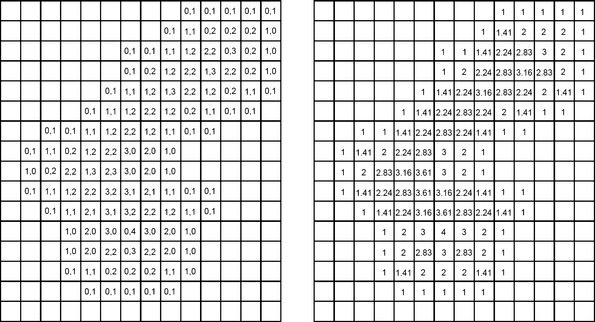
FIGURE 3.12 Computation of the Euclidean distance transform. Left: the pair of (final) values at a pixel of ![]() are its x and y coordinate differences from the nearest pixel of
are its x and y coordinate differences from the nearest pixel of ![]() . Right: corresponding values of the Euclidean distance, rounded to two decimal places.
. Right: corresponding values of the Euclidean distance, rounded to two decimal places.
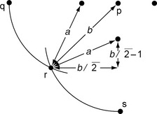
To see how the distances computed by Danielsson’s algorithm can be incorrect, consider circles of radius a centered at (x − 1, y) and (x, y −1) (see Figure 3.13). Let q =(x – a − 1, y) and s = (x, y – a −1), and let r be the point where the circles intersect. If q, r, and s are in, the algorithm gives value a+ 1 to the pixel p at (x,y), because its neighbors (x – 1,y) and (x,y −1) are at distance a from q and s, respectively; however, p is actually at distance b <a + 1 from r. Indeed, as we see from Figure 3.13, the distance a from (x, y−1) to r is the hypotenuse of a right triangle with legs that are b/![]() and (b/
and (b/![]() ) − 1; thus a2 = b2/2+ (b2/2)+1 – b/
) − 1; thus a2 = b2/2+ (b2/2)+1 – b/![]() = b2 –
= b2 –![]() , so that the following is true:
, so that the following is true:
It can be shown that this is a worst case; note that even in this case the error is only a fraction of the grid constant.
3.4.4 Medial axes
For any grid metric dα, any pixel p, and any k ≥ 0, let P(k)(p) = {q : dα(p,q) ≤ k}; thus P(0)(p) = {p}⊂ P(1)(p) ⊂ P(2)(p) ⊂ …. We recall that, for α = 4, P(k)(p) is a diagonally oriented square centered at p, and, for α = 8, P(k)(p) is an upright square centered at p. If p ∈ ![]() and k <dα(p,
and k <dα(p, ![]() ), evidently P(k)(p) ⊆
), evidently P(k)(p) ⊆ ![]() , and all of the P(k)(p)s contain p,so
, and all of the P(k)(p)s contain p,so ![]() is the union of all balls P(k)(p) with p ∈
is the union of all balls P(k)(p) with p ∈ ![]() and k <dα (p,
and k <dα (p, ![]() ).
).
In the dα distance transform of P, each pixel p of ![]() has value dα(p,
has value dα(p, ![]() ). Evidently, Pdα (p,
). Evidently, Pdα (p, ![]() )) (p) is not contained in P (dα(q,
)) (p) is not contained in P (dα(q,![]() )) (q) for any neighbor q of p iff p ∈ Mα
)) (q) for any neighbor q of p iff p ∈ Mα![]() . Hence
. Hence ![]() is the union of the balls (dα (q,
is the union of the balls (dα (q,![]() ))(p) for all p ∈ Mα(
))(p) for all p ∈ Mα(![]() ). The picture in which the value of p is dα (p,
). The picture in which the value of p is dα (p, ![]() ) if p ∈ Mα (
) if p ∈ Mα (![]() ) and 0 otherwise is called the dα medial axis transform (MAT) of
) and 0 otherwise is called the dα medial axis transform (MAT) of ![]() .
.
Definition 3.3
We say that p belongs to the medial axis Mα(![]() ) of
) of ![]() if dα(p,
if dα(p,![]() ) is a local maximum of the dα distance transform of P (i.e., dα(q,
) is a local maximum of the dα distance transform of P (i.e., dα(q, ![]() ) ≤ dα(p,
) ≤ dα(p, ![]() ) for all α-neighbors q of p).
) for all α-neighbors q of p).
The medial axis transforms for the distance transforms of Figures 3.10 and 3.12 are shown in Figure 3.14. Note that the pixels of Mα(![]() ) are centrally located in
) are centrally located in ![]() , so they constitute a kind of “skeleton” of
, so they constitute a kind of “skeleton” of ![]() ; however, this skeleton may not be connected even if
; however, this skeleton may not be connected even if ![]() is simply connected, and it may be two pixels thick if
is simply connected, and it may be two pixels thick if ![]() has even width. Methods of constructing thin connected skeletons will be discussed in Section 16.3.
has even width. Methods of constructing thin connected skeletons will be discussed in Section 16.3.

FIGURE 3.14 Medial axis transforms for the distance transforms of Figures 3.10 and 3.12. Left: d4. Center: d8. Right: approximate de (values shown to one decimal place).
For any p ∈ ![]() and any grid metric dα, let Dα(p) be the largest ball P(k)(p) centered at p that is contained in
and any grid metric dα, let Dα(p) be the largest ball P(k)(p) centered at p that is contained in ![]() . If p ∈ Mα(
. If p ∈ Mα(![]() ), Dα(p) can be α-adjacent to
), Dα(p) can be α-adjacent to ![]() at only one pixel. For example, let
at only one pixel. For example, let ![]() be a “vertical strip” of even width; then Mα is of width 2, and the largest balls “touch” the strip’s border on only one side, at a
be a “vertical strip” of even width; then Mα is of width 2, and the largest balls “touch” the strip’s border on only one side, at a
single border pixel. Thus p ∈ Mα (![]() ) implies only that there is at least one shortest α-path from p to
) implies only that there is at least one shortest α-path from p to ![]() . The original definition of M(
. The original definition of M(![]() ) described the process of constructing M(
) described the process of constructing M(![]() ) in terms of a “grass fire” ignited along the border of
) in terms of a “grass fire” ignited along the border of ![]() and defined M(
and defined M(![]() ) as the locus of points at which the grass fire meets itself. However, as we have seen, a pixel on the medial axis is not necessarily characterized by two shortest α-paths from p to
) as the locus of points at which the grass fire meets itself. However, as we have seen, a pixel on the medial axis is not necessarily characterized by two shortest α-paths from p to ![]() . (This is true also in the continuous case, for example, for a parabolic set, where the endpoint of the medial axis is at distance 0 only from itself.) On the other hand, if there are at least two shortest α-paths from p to
. (This is true also in the continuous case, for example, for a parabolic set, where the endpoint of the medial axis is at distance 0 only from itself.) On the other hand, if there are at least two shortest α-paths from p to ![]() , then p is on the medial axis.
, then p is on the medial axis.
Our definitions of the distance transform and the medial axis transform assumed that P is a binary picture. We conclude this section by mentioning several generalizations of the medial axis transform to multivalued pictures.
In the SPAN [7], P is approximated by a set of maximal “disks” (e.g., squares) in which the pixel values are “homogeneous,” and the generalized medial axis is the set of centers of the disks. If P is binary, the disks have constant value 1, the approximation is exact, and the set of centers of the disks is M(P). (A medial axis based on fuzzy disks [fuzzy sets with membership, that depend only on distance from an origin] is described in [792].)
In the GRAYMAT [644], the gray-weighted length of a path is defined as proportional to the sum of the values of the pixels on the path (see Section 3.4.1), and the generalized medial axis is the set of pixels p that do not lie on any minimal-length path from any other pixel to the set of 0s.
The GRADMAT [1118] assigns a score to a pixel p by summing the gradient magnitudes (the maximal rates of change) of the pixel values at pairs of pixels that have p as their midpoint; the generalized medial axis consists of pixels that have high scores. Note that, in a binary picture, the gradient of the pixel values is nonzero only at the frontier of 〈 P 〉 .
A definition of the medial axis based on morphologic operations will be given in Section 15.6.3; this definition too applies to multivalued pictures.
3.5 Exercises
1. Let p = (x1, y1, z1) and q =(x2, y2, z2) be points in R3, and let the following be true:
Prove that dt is not a metric on R3 but rather that it is a metric on the subset {p : p =(x,y,z)∈ R3 Λ z ≥ 0}. We call it the forest metric, because it corresponds to the distance in which moves are of the form “climb down the first tree, walk to the second tree, and climb up the second tree.”
2. Prove that d has properties M1 through M3 on S iff it has the following two properties:
3. Let [S,d] be a metric space. A sequence {pi}i = 0,1,2 of points of S is called convergent iff there is a p ∈ S such that, for any ε bsol; 0, there is an i0∈ N such that pi ∈ Uε(p) for all i ≥ i0. It is not hard to see that p must be unique; it is called the limit point of the sequence. Show that a sequence pi = (xi, yi)∈ R2 (i = 0,1,2,…) is convergent in [R2,Lm](1 ≤ m ≤∞) iff it is convergent in [R2,de].
4. Is the sequence 1,−2,3,–4,…,… convergent in [R,de]∈ Are the sequences
convergent in [R2,de]∈ Are they convergent if we use the binary metric db∈ If so, what are their limit points∈
5. Let C be a disk of integer radius centered at a grid point, and let D be the frontier of the union of the grid cells that are contained in C. Prove that the Hausdorff distance between the frontiers of C and D is equal to the grid constant.
6. Prove that d4 and d8 are metrics on Z2.
7. Prove that, on a (k+ 1)×(k+ 1) grid, de–d8 can be as great as (![]() . − 1)k ≈ 0·41k and d4 – de can be as great as (2 –
. − 1)k ≈ 0·41k and d4 – de can be as great as (2 –![]() )k ≈ 0.59k. Prove that, for the “octagonal” distance d (Equation 3.11), we have |de – d|≤ (
)k ≈ 0.59k. Prove that, for the “octagonal” distance d (Equation 3.11), we have |de – d|≤ (![]() /2 − 1)k ≈ 0.12k.
/2 − 1)k ≈ 0.12k.
8. Let pm be the norms defined in Section 3.1.2. Prove that, for any p ∈ R2,we have p||2 ≤ p1 ≤ p2, p∞ p2 ≤ p∞, and p∞ ≤ p1 ≤ 2p∞. Express these inequalities in terms of the metrics d4, de and d8 on R2. For R3, prove that d26(p, q) ≤ de(p, q) ≤ · d26(p, q) and de(p, q) ≤ d6(p, q) ≤ · de(p, q).
9. Define “hyperoctagonal” distances d by combining d6 with d18 or d26, and find bounds on |de – d| on a (k+ 1)×(k+ 1) grid.
10. The 3D grid is composed of grid planes z = k, where k is an integer. Construct a modified grid in which odd-numbered grid planes are shifted half a unit in the+ x and+ y directions. Each point in this grid can be regarded as having 12 neighbors: four on its own plane and four on each of the planes above and below it. Define a “d12” metric on this grid in analogy with the dh metric on the hexagonal 2D grid defined in Section 3.2.3.
11. Prove that d1,1 = d8 and d1,∞ = d4.
12. Prove that the following is true:
Prove that the chamfer distance d1,b that best approximates de has b = (1/)+ −1 ≈ 1.351 and that, for this d1,b, we have the following:
This optimal b is close to 4/3; we therefore get a good approximation to 3de by using a = 3 and b = 4 (“(3,4) chamfer distance”). (Other simple combinations of basic moves can be used to give even better approximations to Euclidean distance.)
13. Find bounds for |de – da,b,c| on a (k+ 1)×(k+ 1)×(k+ 1) grid where da,b,c is a 3D chamfer distance, and find values for a, b, and c that minimize these bounds.
14. A knight in chess can move two steps in an isothetic direction and one step in a perpendicular direction. For any p,q ∈ Z2, let dk (p, q) be the minimum number of knight’s moves required to go from p to q. Prove that dk is a metric on Z2.
15. Define a concept of intrinsic distance for fuzzy subsets. (Hint: Define the length of a path (p1,…, pn) as the sum of f (μ(pi)) where f is a monotonic function that maps 0 into∞ and 1 into 0.)
16. An integer-valued picture P is called α-smooth iff |P(p) – P(q)| ≤ 1 whenever p and q are α-neighbors. Prove that the dα distance transform of a binary picture P is the lowest-valued α-smooth picture that has value 0 at all pixels of ![]() .
.
17. Give a “two-scan” algorithm for computing the value-weighted distance from every non-0 to the set of 0s in a multivalued picture.
18. Give “two-scan” algorithms for computing 3D distance transforms for d6, d18, and d26.
19. Give an algorithm for computing a 3D Euclidean distance transform.
20. Prove that p ∈ Mα(P) iff p does not lie on a shortest α-path from any q ≠ p ∈ to ![]()
![]() .
.
21. Define algorithms analogous to those in Theorem 3.8 for constructing the binary picture with a set of 1s that is ![]() given the medial axis transform of P.
given the medial axis transform of P.
22. An oval is a bounded closed convex subset of R2; it is said to be proper if it has interior points. Two sets do not overlap iff their interiors are disjoint. Let M be a proper oval, and let n(M) denote the maximum number of nonoverlapping translates of M that can be arranged so as not to be disjoint from M. Prove that 7 ≤ n(M) ≤ 9, and show that n(M) = 7 if M is a disk and n(M) = 9 if M is a square.
23. Design an efficient algorithm for calculating the intrinsic diameter of a simple polygon or polyhedron and the intrinsic distances between pairs of its vertices.
24. Prove that the intrinsic (4- or 8-)diameter of a connected set of pixels S (the greatest intrinsic [4- or 8-]distance between any two pixels of S) is at most half the total (4- or 8-)perimeter of S (the sum of the [4- or 8-]perimeters of all of the frontiers of S).
3.6 Commented Bibliography
There are many textbooks about metric, normed, and Hilbert spaces; see, for example, [144, 490, 1071]. For relationships between topologies and metrics, see [352]. For a survey of publications about digital metrics, see [720].
Metrics on Z2 were studied in [922], which is the source of Proposition 3.2. The integer-valued metrics d4 and d8, the “octagonal” metrics obtained by combining d4 and d8, and the “hexagonal” metric dh were all introduced in [922]; an improved treatment of dh was given in [672]. For characterizations of d4 and d8, see [411, 718, 719, 723, 850] and [284]; for rounded Euclidean distance, see [851]; for additional results about octagonal distances, see [243, 244, 752].
Metric d18 was defined and studied in [785]. [365] also calculates d18 and counts the number of all minimum-length 18-paths between the origin and a grid point (i,j,k)∈ Z3. For other references about numbers of paths, see [235, 241, 365, 922].
The n-dimensional case (see Section 3.3) was treated in [540]. The metrics∂α on ![]() ,0 ≤α <n (see Theorem 3.6 and Equation 3.15) define balls (all n-cells at distances ≤ r ∈ N from the origin) and spheres (all n-cells at distance = r ∈ N from the origin). [242] studied the volumes of these balls and the “surface areas” of these spheres (the numbers of n-cells contained in the ball or sphere).
,0 ≤α <n (see Theorem 3.6 and Equation 3.15) define balls (all n-cells at distances ≤ r ∈ N from the origin) and spheres (all n-cells at distance = r ∈ N from the origin). [242] studied the volumes of these balls and the “surface areas” of these spheres (the numbers of n-cells contained in the ball or sphere).
For metrics defined by arbitrary neighborhood sequences, see [233, 239, 1146, 1147]. Chamfer distances in arbitrary dimensions were popularized in [103]. See [104, 108, 182, 236, 237, 238, 239, 241, 245, 526, 701, 785, 852, 1037] for related work. For criteria for optimizing chamfer distances, see [66, 67, 107, 156, 1093, 1114]. Distance functions were used to define “continuous” functions on pictures in [767, 903]. For linear metrics on discrete sets, see [247]. For metric-preserving transforms, see [233].
For geodesic distances, see [619]; for geodesic distances on fuzzy subsets, see [91]. Much of the material in Section 3.2.4 is from [889]. Average distances in digital sets are studied in [904], and metric bases in the grid are studied in [724]. [525] estimates distances between borders of components of voxels by calculating geodesics that contain only border voxels.
See [63] for properties of the Hausdorff metric on compact sets. The algorithm discussed in Section 3.2.5 was proposed in [989]. For a linear-time algorithm for calculating the Hausdorff distance between convex polygons, see [52]. The maximum Euclidean distance between two finite planar sets can be calculated in O(n log n) time [1063]. Algorithms for calculating Hausdorff distances (defined by arbitrary Minkowski metrics) between finite planar sets are discussed in [457]. Distances between sets (as in Proposition 3.4) were studied in [556] under the name measures of correspondence. Minimization of the Hausdorff distance between a bounded set S ⊂ Rn and a set M ⊂ Zn defines the Hausdorff digitization of S; see [131, 1116]. See [458] for more about distances between pictures. Hausdorff distances between fuzzy sets (or multilevel pictures) are studied in [179, 181, 901].
For a generalization of the concept of a distance transform, see [897]. The two-scan algorithm for computing the d4 and d8 transforms was introduced in [921], which also introduced the digital medial axis (under the name “distance skeleton”). This was further explored in [933]. For fast computation of distance transforms, see [833]. Generalized distance transforms are discussed in [1119]. For computing distance and distance-related transforms in nonrectangular domains, see [818]. For constrained distances, see [1095]. For 3D distance transforms and their uses, see [1040]. For other references about distance transforms, see [520, 929, 977]. [224] contains a detailed review of distance transforms and also covers algorithmic and application aspects.
The generalization of distance transforms to multivalued pictures (using the value-weighted distance to the set of pixels that have value 0) was studied in [644]. For the computation of such transforms, see [880]; for other weighted distances, see, for example, [92, 829, 1011, 1054, 1057]. For fuzzy distance transforms, see [945].
Algorithms for computing Euclidean distance transforms are discussed in [103, 125, 225, 229, 304, 306, 647, 754, 982, 983, 987]. Figure 3.13 and the accompanying discussion follows [229]. Other references for Euclidean distance transforms are [115, 263, 608, 717, 745, 831, 832, 1010, 1097]. For the 3D case, see [834, 1056, 1068].
For the medial axis (also called the “symmetric axis”) and its mathematic theory, see [93, 160, 707]. For other references about digital medial axes, see [2, 28, 34, 40, 85, 197, 199, 200, 213, 322, 349, 476, 521, 634, 686, 774, 777, 953, 972, 956, 975, 1038, 1142]. For medial axes for chamfer and Euclidean distances, see [39, 41, 42, 303, 359, 845, 846, 953, 984, 1094, 1133].
For the “knight’s distance” (Exercise 10), see [240, 244]. Exercise 22 is from [394], and Exercise 24 is from [886].
1The norm ![]() is defined not only for integer m but for any real number m ≥ 1.
is defined not only for integer m but for any real number m ≥ 1.
2In the mathematics literature, a unit circle or unit sphere is traditionally defined as having radius 1 (i.e., diameter 2), whereas a unit square or unit cube is (inconsistently!) defined as having side 1.
3Intrinsic distance is sometimes called “geodesic distance,” but, to avoid confusion with the noun “geodesic,” we will not use that term.
4The distance transform is essentially the same as the distance field F(![]() ); see Section 3.2.5.
); see Section 3.2.5.