
Topology
Digital geometry is often concerned with analyzing topologic properties of sets of pixels or voxels. The topology of Euclidean space was briefly discussed in Section 3.1.7. The definitions of open and closed regions in Section 5.1.4 indicated that these topologic concepts are applicable to discrete structures. This chapter summarizes basic topologic concepts and properties that are relevant to adjacency and incidence grids, defines digital topologies, and provides a brief introduction to combinatorial topology.
6.1 Topologic Spaces
In the last third of the 19th century, H. Poincaré and others established topology as a branch of modern mathematics. Point-set topology studies topologic spaces. In early publications about topology, the underlying set S of a topologic space was a Euclidean space, but, in modern topology, it can be an abstract set.
6.1.1 General definitions
[S, G] is called a topologic space iff G is a family of subsets of S that has the following three properties:
T2: Let M1, M2,… be a finite or infinite family of sets in G; then the union of these sets is also in G.
T3: Let M1, M2,…, Mn be a finite family of sets in G; then the intersection of these sets is also in G.
G is called a topology on S, and its elements are called open sets. M ⊆ S is called closed iff its complement ![]() is open. It follows from T2 and T3 that the family of closed subsets of S is closed under finite unions and arbitrary intersections.
is open. It follows from T2 and T3 that the family of closed subsets of S is closed under finite unions and arbitrary intersections.
The interior M° of M ⊆ S is the union of all open subsets of M. The closure M• of M is the intersection of all closed subsets of S that contain M. Set M is open iff it coincides with its interior and closed iff it coincides with its closure. ![]() is called the frontier of M.
is called the frontier of M.
The degenerate topology ![]() , in which every subset of S is open as well as closed, is a topologic space. In this topology, we have M• = M° = M and ∂M = ø for every M ⊆ S. (The degenerate topology is called the “discrete topology” in most books about topology, but this would not be appropriate in a book about digital geometry.)
, in which every subset of S is open as well as closed, is a topologic space. In this topology, we have M• = M° = M and ∂M = ø for every M ⊆ S. (The degenerate topology is called the “discrete topology” in most books about topology, but this would not be appropriate in a book about digital geometry.)
Any metric space [S,d] induces a topology on S; see Section 3.1.7. In this topology, the closure M* is the set of all p ∈ S such that d(p, M) = 0.
The Euclidean metric de induces the Euclidean topology ![]() on
on ![]() (n ≥ 1). For example, for n = 1, an open interval (x,y) = {z ∈
(n ≥ 1). For example, for n = 1, an open interval (x,y) = {z ∈ ![]() : x <z < y} (x,y ∈
: x <z < y} (x,y ∈ ![]() ; x <y) is an open set, and a closed interval [x,y] = {z ∈ :
; x <y) is an open set, and a closed interval [x,y] = {z ∈ : ![]() x ≤ z ≤ y} is a closed set.
x ≤ z ≤ y} is a closed set.
The binary metric db induces the degenerate topology on any set S. The metrics dα, α ∈ {4,6,8,18,26} (see Section 3.2.2) and∂α, α ∈ {0,1,2} (see Section 3.3.1) also induce the degenerate topology on ![]() or
or ![]() (the grid point model) and on
(the grid point model) and on ![]() (the grid cell model).
(the grid cell model).
Nondegenerate topologies can be defined on discrete sets. In particular, the open sets of Section 5.1.4 define a topology on any incidence pseudograph. We will discuss these topologies in detail later in this chapter.
Let [S, G] be a topologic space and M ⊆ S; then [M, GM] is also a topologic space, where GM = {A ∩ M : A ∈ Z}. GM is called the inherited topology on M, and M is called a topologic subspace of S. Note that M itself is both open and closed in GM. (The inherited topology is also called “relative topology” in topology textbooks.)
Maximum connected subsets of M are called components of M.
[S, G] is called an Aleksandrov1 space or Aleksandrov topology iff any intersection of open sets is open. If S is finite, any [S, G] is Aleksandrov.
For example, in the Euclidean topology ![]() 1 on
1 on ![]() , an open interval (x,y) is a neighborhood of any z ∈ (x,y), and a closed interval [x,y] is a neighborhood of z ∈ [x,y] iff z ≠ x and z ≠ y.
, an open interval (x,y) is a neighborhood of any z ∈ (x,y), and a closed interval [x,y] is a neighborhood of z ∈ [x,y] iff z ≠ x and z ≠ y.
In an Aleksandrov space, the intersection U (p) of all neighborhoods of p ∈ S is the smallest neighborhood of p, which is also called the star of p. Evidently, U (p) must be an open set. U may not define a symmetric relation on S; we can have q ∈ U (p) but ![]() .
.
[S, G] is called a Kolmogorov space or T0-space iff, for any two distinct points of S, at least one of them has a neighborhood that does not contain the other.2 The degenerate topology is a T0-space. An Aleksandrov topology is T0 iff, for every two distinct points p and q, U(p) and U(q) are distinct.
For example, in the topology induced by a metric space, the set of all ε -neighborhoods is a basis. The set of all open intervals of ![]() is a basis of the Euclidean topology
is a basis of the Euclidean topology ![]() 1. In an Aleksandrov topology, the set of all smallest neighborhoods is a basis.
1. In an Aleksandrov topology, the set of all smallest neighborhoods is a basis.
Example 6.1
(N. Bourbaki, 1961) The family {[x, +∞): x ∈ ![]() } is a basis of a topology on
} is a basis of a topology on ![]() called the right topology on
called the right topology on ![]() . It follows, for example, that any (–∞, x) is closed. Analogously, the family {(−∞, x] : x ∈
. It follows, for example, that any (–∞, x) is closed. Analogously, the family {(−∞, x] : x ∈ ![]() } is a basis of a topology on
} is a basis of a topology on ![]() called the left topology on
called the left topology on ![]() . Note that the sets [x, +∞) and (−∞,x] are not open in the Euclidean topology on
. Note that the sets [x, +∞) and (−∞,x] are not open in the Euclidean topology on ![]()
A topologic space has a countable basis iff it has a basis of cardinality of at most N0, where N0 is the cardinality of the set ![]() of natural numbers. For example, the set of all open intervals with rational endpoints is a countable basis of
of natural numbers. For example, the set of all open intervals with rational endpoints is a countable basis of ![]() 1.
1.
6.1.2 Poset topologies
A reflexive, antisymmetric (for all pairs p and q such that p ≠ q), transitive binary relation on a set S is called a partial order and is denoted by ![]() . [S,
. [S,![]() ] is called a partially ordered set (poset, for short).
] is called a partially ordered set (poset, for short).
Definition 6.4
In the poset topology on ![]() , M ⊆ S is open iff p ∈ M and
, M ⊆ S is open iff p ∈ M and ![]() implies q ∈ M for all p,q ∈ S.
implies q ∈ M for all p,q ∈ S.
Any poset topology is Aleksandrov. Following [9], we know that there is a one-to-one correspondence between Aleksandrov topologies on a set S and quasiorders (reflexive and transitive relations) on S, and a quasiorder is a partial order iff the corresponding Aleksandrov topology is T0. An open set defines an “upper set” of the quasiorder (in the sense of Definition 6.4), and the order “less than or equal to” corresponds to “is in the closure of.”
The incidence grid topology (see Section 6.2.3) is an example of a poset topology. Another example is the following:
In this example, {i}⊆{i}, {i,i + 1}⊆{i,i + 1}, {i}⊆{i,i + 1}, and {i + 1}⊆{i,i + 1} are the only instances of the partial order ![]() . This
. This ![]() is a T0-space. In this topology, {{i, i + 1}} and {{i}, {i, i + 1}, {i, i −1}} are open. The union of the open sets {{2,3}, {3}, {3,4}} and {{4,5}, {5}, {5,6}} is the open set {{2,3}, {3}, {3,4}, {4,5}, {5}, {5,6}}. The union of the open sets {{i}, {i, i + 1}, {i, i −1}} such that i ≤ 2 or i ≥ 6 is the open set
is a T0-space. In this topology, {{i, i + 1}} and {{i}, {i, i + 1}, {i, i −1}} are open. The union of the open sets {{2,3}, {3}, {3,4}} and {{4,5}, {5}, {5,6}} is the open set {{2,3}, {3}, {3,4}, {4,5}, {5}, {5,6}}. The union of the open sets {{i}, {i, i + 1}, {i, i −1}} such that i ≤ 2 or i ≥ 6 is the open set ![]() /{{4}}. The complement of this open set is the closed set {{4}}. Let us consider the following sets (i ∈
/{{4}}. The complement of this open set is the closed set {{4}}. Let us consider the following sets (i ∈![]() , k ≥ 1):
, k ≥ 1):
Cik = {{i},{i,i + 1},{i + 1}, …, {i + k − 1},{i + k − 1,i + k},{i + k}}
The sets {{i}, {i, i + 1}, {i, i −1}}, and {{i, i + 1}} (i ∈ are a countable basis of) are a countable basis of ![]() . M = {{i}, {i + 1}, {i, i + 1}}, which is neither open nor closed in
. M = {{i}, {i + 1}, {i, i + 1}}, which is neither open nor closed in ![]() , has the following inherited topology,
, has the following inherited topology,
GM = {ø,{{i,i + 1}},{{i},{i,i + 1}},{{i + 1},{i,i + 1}},M}
in which the closed sets are as follows:
{ø,{{i}},{{i + 1}},{{i},{i + 1}},M}
Thus M is connected, because it is not a union of two disjoint nonempty closed sets.
6.1.3 Topologies on incidence pseudographs
Let [S,I, dim] be an n-incidence pseudograph. The set of all open subsets of S (consisting of nodes of any dimension) defines a topology on S. Our particular interest is in components that consist of principal nodes. A complete subset M ⊆ S is not always a union of components, because there may be i-nodes in M that are not incident with any n-node in M. M is called purely n-dimensional iff it is a union of components.
Theorem 6.1
The family of purely n-dimensional complete open subsets of S defines a topology G on S. The family of open regions is a basis of this topology.
Proof S andø are complete, purely n-dimensional, and open (and closed). By deMorgan’s rules we have the following, where the index set is finite or countably infinite:
Let Mi be closed, purely n-dimensional, and complete. Then c ∈ Mi, c′ ∈ I(c), and, let dim(c’) < dim(c) imply c’ ∈ Mi. If c is in all of the Mis, c′ is also in all of the Mis; hence the family of purely n-dimensional complete closed subsets of S is closed under arbitrary intersections. The family of purely n-dimensional complete open sets, which are the complements of purely n-dimensional complete closed sets, is therefore closed under arbitrary unions. Let M1,…, Mm be purely n-dimensional complete closed sets. For any c in any Mi, any c′ ∈ I(c) with dim(c′) < dim(c) is also in Mi, and hence is in their union; hence the family of purely n-dimensional complete closed sets is closed under finite unions.
Because S is an incidence structure, it is countable; hence any purely n-dimensional complete open set M ⊂ S is the union of countably many pairwise disjoint components, each of which can be finite or countably infinite. Let C be one of the components, let c ∈ C be an i-node (0 ≤ i <n), and let the following be true:
U(c) = {c′ : c′ ∈ I(c) ∧ dim(c′) ≥ dim(c)}
U(c) is a subset of C by the definition of a closed set. By property I5, there is at least one n-node in each U(c). It follows that every U(c) is an open region and that C is the (finite or countable) union of these regions.
Let M be a purely n-dimensional complete subset of S. Then the following is true where the frontier ∂M and interior M° are defined by the topology G of Theorem 6.1:

6.2 Digital Topologies
In this section, we define digital topologies on sets of grid points or grid cells. We will see in Section 6.2.4 that there exist very few digital topologies on grid point or grid cell spaces of dimension ≤3.
6.2.1 General definition
[S, G] is called a digital topology in the grid cell model iff ![]() and G is a family of open sets that satisfies T1 through T3, as well as the following:
and G is a family of open sets that satisfies T1 through T3, as well as the following:
(A singleton is a set of cardinality 1.) These properties exclude, for example, the degenerate topology ![]() , in which every set that contains at least two pixels is disconnected.
, in which every set that contains at least two pixels is disconnected.
In the grid point model, let d be a metric on ![]() (n ≥ 1), and let Ad(p) = {q : q ∈
(n ≥ 1), and let Ad(p) = {q : q ∈ ![]() ∧ d(p,q) = 1}. A subset of
∧ d(p,q) = 1}. A subset of ![]() is called connected with respect to d iff it is connected with respect to the adjacency relation Ad. [
is called connected with respect to d iff it is connected with respect to the adjacency relation Ad. [![]() , G] is called a digital topology in the grid point model if S =
, G] is called a digital topology in the grid point model if S = ![]() (n ≥ 1), and G is a family of open sets that satisfies T1 through T3, as well as the following:
(n ≥ 1), and G is a family of open sets that satisfies T1 through T3, as well as the following:
D1: All connected sets are connected with respect to L∞.
D2: All disconnected sets are disconnected with respect to L1.
D3: The closure of any singleton is connected with respect to L1.
It can be shown that, in the 2D grid point space, D1 and D2 imply D3.
6.2.2 The grid point topology
Let p = (x1,…, xn) ∈ ![]() (n ≥ 1), and let η1 (p) be the smallest nontrivial neighborhood of p with respect to the Minkowski metric L1 on
(n ≥ 1), and let η1 (p) be the smallest nontrivial neighborhood of p with respect to the Minkowski metric L1 on ![]() (see Section 3.2.2). Define the following:
(see Section 3.2.2). Define the following:
We call p an odd (even) grid point if x1 + …. + xn is odd (even). Note that the relation UGP is asymmetric on ![]() .
.
{Ugp (p): p ∈ ![]() } is a countable basis of a topology that we call the grid point topology [
} is a countable basis of a topology that we call the grid point topology [![]() , UGP]. For example, for n = 1, this basis consists of the sets {2i + 1} and {2i − 1, 2i, 2i + ≥ 1). This topology is called the alternating topology on
, UGP]. For example, for n = 1, this basis consists of the sets {2i + 1} and {2i − 1, 2i, 2i + ≥ 1). This topology is called the alternating topology on ![]() . It is sketched in Figure 6.1.
. It is sketched in Figure 6.1.

UGP defines an adjacency relation AGP on ![]() : p,q ∈ AGP iff p∉q and p ∈ UGP(q) or q ∈ UGP(p). It is not hard to see that AGP = A4 if n = 2 (see Figure 6.2) and AGP = A6 if n = 3. This topology is an Aleksandrov space and a T0-space.
: p,q ∈ AGP iff p∉q and p ∈ UGP(q) or q ∈ UGP(p). It is not hard to see that AGP = A4 if n = 2 (see Figure 6.2) and AGP = A6 if n = 3. This topology is an Aleksandrov space and a T0-space.

FIGURE 6.2 A directed graph showing the asymmetric neighborhood relation UGP for n = 2. Loops (corresponding to the reflexivity of UGP) are omitted.
Theorem 6.2
The grid point topology on ![]() (n ≥ 1) is a digital topology.
(n ≥ 1) is a digital topology.
Proof M ⊂ ![]() is connected iff it is not the union of two disjoint nonempty closed sets in the induced topology on M. It is not hard to see that M is (topologically) connected iff it is connected with respect to L1. It follows that the grid point topology has properties D1 through D3.
is connected iff it is not the union of two disjoint nonempty closed sets in the induced topology on M. It is not hard to see that M is (topologically) connected iff it is connected with respect to L1. It follows that the grid point topology has properties D1 through D3.
Open and closed sets, the interior and closure of a set, and the frontier of a set (the difference between its closure and its interior) can all be defined in the grid point topology. For example, any set that contains an even grid point and at most three of its 4-neighbors (which are odd grid points) is not open, and any set that contains only even grid points is closed.
Figure 6.3 shows two embeddings of the 2D grid point topology into the plane for which the odd grid points map onto the pixel positions in a regular orthogonal grid. Figure 6.4 is based on the embedding shown on the left in Figure 6.3. It shows on the left the two possible configurations of the smallest neighborhood of an even grid point and on the right an example of a closed set. In accordance with the definition of complete subsets of incidence pseudographs (see Section 5.1.1), we can define complete subsets of ![]() in the grid point topology; an even grid point must be in such a subset if its smallest neighborhood is in the subset.
in the grid point topology; an even grid point must be in such a subset if its smallest neighborhood is in the subset.
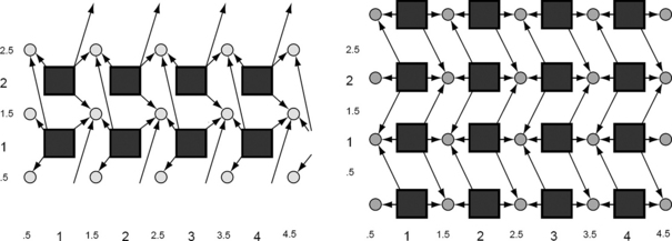
FIGURE 6.3 Two embeddings of the grid point topology into the plane such that the odd grid points (shown as squares) are in pixel positions

FIGURE 6.4 Left: the smallest neighborhoods of even grid points. Right: an example of a closed set. Both are for the embedding shown in Figure 6.3 on the left.
Let ds be the graph metric defined by a switch state matrix S on ![]() (see Section 2.1.3). The relation of s-adjacency defines sets As(p) = {q ∈
(see Section 2.1.3). The relation of s-adjacency defines sets As(p) = {q ∈ ![]() : ds(p,q) = 1}. Let the following be true:
: ds(p,q) = 1}. Let the following be true:
The family of sets Us(p), p ∈ ![]() , is not the basis of a topology on
, is not the basis of a topology on ![]() . To see this, consider h-adjacency, which is an example of an s-adjacency, and consider two “diagonally adjacent” even grid points p and q. Us(p) ∩ Us(q) contains exactly four grid points and so is not one of the sets Us (p). If r is another even grid point “diagonally adjacent” to p, we have Us(p) ∩ Us(q) ∩ Us(r) = {p}. It follows that all subsets of
. To see this, consider h-adjacency, which is an example of an s-adjacency, and consider two “diagonally adjacent” even grid points p and q. Us(p) ∩ Us(q) contains exactly four grid points and so is not one of the sets Us (p). If r is another even grid point “diagonally adjacent” to p, we have Us(p) ∩ Us(q) ∩ Us(r) = {p}. It follows that all subsets of ![]() are open, so the family of sets Us(p) is a basis for the degenerate topology in which only singletons are connected.
are open, so the family of sets Us(p) is a basis for the degenerate topology in which only singletons are connected.
6.2.3 The grid cell topology
The incidence grid [![]() , I, dim](n ≥ 1) defines a poset [
, I, dim](n ≥ 1) defines a poset [![]() , ≤] such that the following is true for all c1, c2 ∈
, ≤] such that the following is true for all c1, c2 ∈ ![]() :
:
c1 ≤ c2 iff c1 ∈ I(c2) ∧ dim(c1) ≤ dim(c2)
The poset topology on [![]() , ≤] is called the grid cell topology. This topology is a T0-space, because it is defined by a partial order. A complete purely n-dimensional subset of
, ≤] is called the grid cell topology. This topology is a T0-space, because it is defined by a partial order. A complete purely n-dimensional subset of ![]() is topologically connected in this topology iff it is connected for the adjacency relation in Definition 5.3. We will see at the end of this section that [
is topologically connected in this topology iff it is connected for the adjacency relation in Definition 5.3. We will see at the end of this section that [![]() , ≤] is a digital topology.
, ≤] is a digital topology.
The star of a cell c is the set of all cells c′ ≥ c; it is the smallest neighborhood of c in the grid cell topology. Figure 6.5 shows examples of stars. The stars are a countable basis of the grid cell topology.
The 2D grid cell topology [![]() , ≤] defines a partition of the plane into grid cells, grid edges, and grid vertices. Figure 2.3 (left) shows a graphic sketch and Figure 2.13 the geometric realization of the 2D incidence grid used throughout this book. P.S. Aleksandrov and H. Hopf used this 2D example in 1935 to illustrate the poset topology.
, ≤] defines a partition of the plane into grid cells, grid edges, and grid vertices. Figure 2.3 (left) shows a graphic sketch and Figure 2.13 the geometric realization of the 2D incidence grid used throughout this book. P.S. Aleksandrov and H. Hopf used this 2D example in 1935 to illustrate the poset topology.
The following is another way of defining a topology on ![]() . We begin by partitioning
. We begin by partitioning ![]() into a countable number of pairwise disjoint intervals. This partition defines a one-to-one mapping
into a countable number of pairwise disjoint intervals. This partition defines a one-to-one mapping ![]() such that, for each i ∈
such that, for each i ∈ ![]() , f−1(i)is a connected subset of
, f−1(i)is a connected subset of ![]() with respect to the Euclidean topology. We then use the Euclidean topology on
with respect to the Euclidean topology. We then use the Euclidean topology on ![]() to induce a topology on
to induce a topology on ![]() based on these intervals. A subset M of
based on these intervals. A subset M of ![]() is open in this topology iff f−1(M) is open in the Euclidean topology on
is open in this topology iff f−1(M) is open in the Euclidean topology on ![]() .
.
The topology induced on ![]() in this way may not be of interest. For example, let f (x) be the integer nearest to x; if x is a half-integer i + ½, let f (x) = i. Then f−1(i) = (i − 2, i + 2) for all i ∈
in this way may not be of interest. For example, let f (x) be the integer nearest to x; if x is a half-integer i + ½, let f (x) = i. Then f−1(i) = (i − 2, i + 2) for all i ∈ ![]() (i.e., f−1(i) is neither open nor closed in
(i.e., f−1(i) is neither open nor closed in ![]() ), and the same is true if we take f (i + ½) = i + 1. As a result, no proper subset of
), and the same is true if we take f (i + ½) = i + 1. As a result, no proper subset of ![]() can be open or closed (i.e., the induced topology on
can be open or closed (i.e., the induced topology on ![]() is the trivial topology that has only the empty setø and
is the trivial topology that has only the empty setø and ![]() itself as open and closed sets). However, we have the following:
itself as open and closed sets). However, we have the following:
Example 6.2
Modify f by defining f (i + ½) as the nearest even integer [503].
This f induces the alternating topology on ![]() (see Figure 6.1). f−1 (2i) is a closed subset of
(see Figure 6.1). f−1 (2i) is a closed subset of ![]() in the Euclidean topology and f−1(2i + 1) is an open subset, so {2i} is a closed subset of
in the Euclidean topology and f−1(2i + 1) is an open subset, so {2i} is a closed subset of ![]() and {2i + 1} is an open subset.
and {2i + 1} is an open subset.
For example, the 2D Euclidean topology is the product of two one-dimensional Euclidean topologies. The topologies on ![]() defined previously can be used to define product topologies on
defined previously can be used to define product topologies on ![]() (n ≥ 2). A product of two Aleksandrov topologies is Aleksandrov, and the corresponding partial order is the product of the two partial orders.
(n ≥ 2). A product of two Aleksandrov topologies is Aleksandrov, and the corresponding partial order is the product of the two partial orders.
The alternating topology is an Aleksandrov space, and so are finite products of alternating topologies. Let UGC(p) be the smallest neighborhood of p ∈ ![]() in such a product topology. (We use the subscript “GC,” because this discussion will lead us back to the grid cell topology.)
in such a product topology. (We use the subscript “GC,” because this discussion will lead us back to the grid cell topology.)
Figure 6.6 shows the asymmetric neighborhood relation UGC in the product of two alternating topologies on ![]() .
.
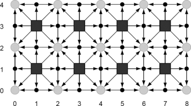
FIGURE 6.6 The asymmetric neighborhood relation UGC. The hollow dots represent closed sets {(2i, 2j)}, the squares represent open sets {(2i + 1, 2j + 1)}, and the solid dots represent sets {(2i, 2j + 1)} or {(2i + 1,2j)}, which are neither open nor closed. Loops (corresponding to the reflexivity of UGC) are not shown.
Theorem 6.3
Finite products of n ≥ 2 alternating topologies are digital topologies on ![]() .
.
Proof We will see in Definition 6.6 how a symmetric adjacency relation AGC can be defined on ![]() by the neighborhood relation UGC. AGC(p) is always contained in A∞(p) = {q : L∞(p,q) = 1} and always contains A1(p) = {q : L1(p,q) = 1}. This implies that D1 through D3 are valid for these product topologies.
by the neighborhood relation UGC. AGC(p) is always contained in A∞(p) = {q : L∞(p,q) = 1} and always contains A1(p) = {q : L1(p,q) = 1}. This implies that D1 through D3 are valid for these product topologies.
M ⊆ ![]() is open in the product of two alternating topologies iff the following is open in
is open in the product of two alternating topologies iff the following is open in ![]() , where f is as it is in Example 6.2:
, where f is as it is in Example 6.2:
Figure 6.7 shows an embedding of this 2D product topology into the plane such that all grid points {(2i + 1,2j + 1)} (shown as squares) are in pixel positions. Figure 6.8 shows on the left the smallest neighborhoods of grid points (compare Figure 6.5) and on the right an example of a closed set. The smallest neighborhood of a grid point (2i + 1, 2j + 1) contains only that point; the smallest neighborhood of a grid point (2i, 2j) is its 8-neighborhood; and all other grid points have smallest neighborhoods of cardinality 3, arranged either horizontally or vertically.

FIGURE 6.7 An embedding of the product of two alternating topologies into the plane such that the open singletons are in pixel positions.

FIGURE 6.8 Left: smallest (topologic) neighborhoods of grid points. Right: an example of a closed set. These figures use the embedding shown in Figure 6.7.
Products of alternating topologies are T0-spaces. For example, the neighborhood of a grid point p = (2i + 1, 2j + 1) does not contain any of the grid points that are 8-adjacent to p.
Proposition 6.1
Any product of n ≥ 2 alternating topologies is homeomorphic (see Definition 6.8) to the n-dimensional grid cell topology [![]() , ≤].
, ≤].
Proof The base set ![]() of the alternating topology consists of an alternating sequence of open integers 2i + 1 and closed integers 2i. The coordinates of a grid point p in the base set
of the alternating topology consists of an alternating sequence of open integers 2i + 1 and closed integers 2i. The coordinates of a grid point p in the base set ![]() of the product topology consist of ap open and bp closed integers such that ap + bp = n. Consider the one-to-one mapping Φ, which maps p ∈
of the product topology consist of ap open and bp closed integers such that ap + bp = n. Consider the one-to-one mapping Φ, which maps p ∈ ![]() into an ap-cell in
into an ap-cell in ![]() such that p ∈ UC(q) iff [Φ (p), Φ (q)] ∈ I and dim(Φ(p)) ≤ dim(Φ(q)). (It is not hard to show that UC and I allow such a one-to-one mapping.)Φ maps open subsets of the product topology into open subsets of the incidence grid, and Φ−1 maps open subsets of the incidence grid into open subsets of the product topology. (In 2D, this follows, for example, from Equation 6.3.) Thus Φ is a homeomorphism between the two topologic spaces.
such that p ∈ UC(q) iff [Φ (p), Φ (q)] ∈ I and dim(Φ(p)) ≤ dim(Φ(q)). (It is not hard to show that UC and I allow such a one-to-one mapping.)Φ maps open subsets of the product topology into open subsets of the incidence grid, and Φ−1 maps open subsets of the incidence grid into open subsets of the product topology. (In 2D, this follows, for example, from Equation 6.3.) Thus Φ is a homeomorphism between the two topologic spaces.
From this and Theorem 6.3, it follows that [![]() , ≤](n ≥ 1) is a digital topology.
, ≤](n ≥ 1) is a digital topology.
6.2.4 The number of digital topologies
There is only one digital topology for n = 1: the alternating topology on ![]() .
.
Theorem 6.4
Let S be a subset of ![]() that contains a translate of the set G0 shown in Figure 6.9. Then there is no topology on S in which connectivity is the same as 8-connectivity.
that contains a translate of the set G0 shown in Figure 6.9. Then there is no topology on S in which connectivity is the same as 8-connectivity.

FIGURE 6.9 The set G0 used in Theorem 6.4.
Let ![]() be a digital topology, and let U(p) be the intersection of all of the open sets of G that contain p. Then, for all p ∈
be a digital topology, and let U(p) be the intersection of all of the open sets of G that contain p. Then, for all p ∈ ![]() , we must have U (p) ⊆ N8(p). If not, the 8-disconnected set
, we must have U (p) ⊆ N8(p). If not, the 8-disconnected set ![]() /A8 (p) would be connected in
/A8 (p) would be connected in ![]() , because any open set containing p would also contain a point in
, because any open set containing p would also contain a point in ![]() /N8(p).
/N8(p).
This result limits the possible topologic neighborhoods U(p) that can be used to define a basis for a digital topology:
It follows that the 2D grid point and grid cell topologies are the only two possible 2D digital topologies.
In addition to the 3D grid point and grid cell topologies, we also have the product of two one-dimensional grid cell topologies and one one-dimensional grid point topology; a topology ![]() in which alternate grid planes have the grid point and grid cell topologies; and a topology with open sets that are the closed sets of
in which alternate grid planes have the grid point and grid cell topologies; and a topology with open sets that are the closed sets of ![]() .
.
The grid point and grid cell topologies exist on ![]() for all n; they are the “most regular” digital topologies.
for all n; they are the “most regular” digital topologies.
Geometric realizations such as those shown in Figures 2.13 and 2.14 are models for the 2D and 3D grid cell topologies; these models can be generalized to n dimensions.3 The grid point topology can also be geometrically represented by a tessellation of the Euclidean plane or space into convex polygons or polyhedra. For example, in Figure 6.10, the squares represent odd grid points (2-cells), and the trapezoids represent even grid points (1-cells); there are no 0-cells in this digital topology.

FIGURE 6.10 Left: geometric representation of the smallest neighborhoods of even grid points. Right: the closed set of Figure 6.4, which is now shown as a union of convex polygons.
The algorithms described in Section 5.4.1 can be used to assign 1-cells to their adjacent 2-cells that have the largest pixel values.
The values of topologic properties of a set M of pixels or voxels depend in general on which digital topology is being used. These values remain the same if the topologic spaces are homeomorphic (see Definition 6.8) and M is interpreted in the same way (e.g., as an open set).
6.2.5 Topologic adjacency and dimension
The concept of a smallest neighborhood U (p) in an Aleksandrov space allows us to define a symmetric adjacency relation on the space (see Section 2.1.4):
This relation defines an adjacency structure [S, A] that does not necessarily satisfy properties A1 through A3 of an adjacency graph. For example, if S is not topologically connected, then [S, A] does not satisfy A2. The degenerate topology is an Aleksandrov space with U (p) = {p} for all p ∈ S; it generates the degenerate adjacency relation A = ø. Obviously, the adjacency relations Aα defined by the metrics dα (α ∈ {4,6,8,18,26}) are not the same as the adjacency relation A = ø in the degenerate topology induced by the metric spaces ![]() (n = 2 or 3). Definition 6.6 relates to Definition 5.2 as follows: let two i-adjacent nodes c1 and c2 both be incident with the i-node c, which differs from both c1 and c2. In the Aleksandrov space [S, ≤], we have two adjacency pairs {c, c1} and {c, c2}, and c1 and c2 are connected via c.
(n = 2 or 3). Definition 6.6 relates to Definition 5.2 as follows: let two i-adjacent nodes c1 and c2 both be incident with the i-node c, which differs from both c1 and c2. In the Aleksandrov space [S, ≤], we have two adjacency pairs {c, c1} and {c, c2}, and c1 and c2 are connected via c.
The smallest neighborhoods UGP and UGC of grid points p ∈ ![]() (n ≥ 2) define adjacency relations AGP and AGC as in Definition 6.6. AGP = A4 in 2D and = A6 in 3D. AGC(p) = A4(p) in 2D iff p has one odd and one even coordinate, and it equals A8(p) otherwise.
(n ≥ 2) define adjacency relations AGP and AGC as in Definition 6.6. AGP = A4 in 2D and = A6 in 3D. AGC(p) = A4(p) in 2D iff p has one odd and one even coordinate, and it equals A8(p) otherwise.
Any adjacency relation on a set S defines paths, connectedness, components, and so forth, as discussed in Sections 1.1.4 and 1.2.5. Let A* (p) be the union of A(p) with all points r ∈ S for which there exist q1,q2 ∈ A(p) such that a shortest A-path from q1 to q2 not passing through p passes through r. For example, ![]() for p ∈
for p ∈ ![]() , and
, and ![]() and
and ![]() for q ∈
for q ∈ ![]() . We have A(c)= A* (c) for any cell c in the grid cell topology.
. We have A(c)= A* (c) for any cell c in the grid cell topology.
A set M is called totally disconnected with respect to adjacency A iff there is no pair of distinct points p, q ∈ M such that {p, q} is A-connected.
Definition 6.7
Let M be a subset of an adjacency structure [S, A] that satisfies property A1. The dimension dimA(M) of M is defined as follows:
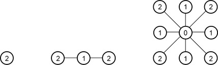
Figure 6.11 shows examples of one- and two-dimensional sets in the 4- and 8-adjacency grids and in the 2D incidence grid.

FIGURE 6.11 Upper row: zero-dimensional subgraphs in the (left) 4-adjacency grid, (middle) 8-adjacency grid, and (right) 2D incidence grid (for topologic adjacency). Middle row: one-dimensional subgraphs. Bottom row: two-dimensional subgraphs.
Proposition 6.2
A 4-connected set M ⊆ ![]() is 2D iff it has a 2 × 2 square of grid points as a proper subset.
is 2D iff it has a 2 × 2 square of grid points as a proper subset.
Proof Let M be a set of four grid points that form a “T”. There exists a grid point p0 such that card(A(p0) ∩ M) = 3 so that case (iii) does not apply. However, from case (iv), we have dimA(A8(p0) ∩ M) = 0, because case (ii) applies; thus dimA(M) = 1. Similarly we can show that dimA(M) ≤ 1 for any set M that does not contain a 2 × 2 square of grid points by considering all possible such M s in a 3 × 3 square of grid points.
If M is a 2 × 2 square of grid points, for any of its four points, we have card (A4(p) ∩ M) = 2; thus case (iii) applies, so dimA(M) = 1.
Finally, suppose M properly contains a 2 × 2 square of grid points. If, for at least one of these points p0 we have card(A4(p0) ∩ M) = 3, we can apply case (iv) to obtain dimA(A8(p0) ∩ M) = 1. Hence, in accordance with case (iv), we have dimA(M)= 2.
Figure 2.20 shows all 4-connected sets of grid points of cardinality 8; the two-dimensional sets (with respect to 4-adjacency) are shown with filled dots.
An elementary grid triangle is a set T = {(i,j), (i + 1, j), (i + j + 1)} or a 90°, 180°, or 270 rotation of it. Such a T is one-dimensional for A4 in accordance with case (iii).
Proposition 6.3
An 8-connected set M ⊆ ![]() is 2D iff it has an elementary grid triangle as a proper subset.
is 2D iff it has an elementary grid triangle as a proper subset.
This proposition can be proved using a case discussion similar to that used in the proof of Proposition 6.2.
In 3D, consider adjacency relation A6, and let M = N26(o) = A26 (o) ∪{o} where o =(0,0,0). Without using the extended set A* in case (iv), we obtain the following:
For any p ∈ M and L = A6(p) ∩ M, L is a totally disconnected nonempty set with respect to A6 so that dimA(L) = 0 and dimA(M) = 1.
Using the extended set A* in Definition 6.7 makes M 3D for A6, A18, and A26. For example, for o ∈ M and L = A18(o) ∩ M, we have card(A18(q) ∩ L) ≥ 4 for any q ∈ L; for example, card(A18(q) ∩ L) = 4 for q =(0,0,1), and card(A18(q) ∩ L) = 6 for q =(1,0,1). By repeated application of case (iv), we obtain the following:
For any p ∈ A18(q) ∩ L, we have dimA(A18(p) ∩ (A18(q) ∩ L)) = 0 using case (ii); hence dimA(A18(q) ∩ L)= 1, dimA(L)= 2, and dimA(M)= 3.
Note that the dimensions of cells in incidence grids ![]() are the dimensions of subsets of
are the dimensions of subsets of ![]() and that the Euclidean topology is not an Aleksandrov space. For example, the countably infinite intersection of the open intervals (−ε, +ε), for all rational ε such that 1 ≥ε> 0, is the closed singleton {0}.
and that the Euclidean topology is not an Aleksandrov space. For example, the countably infinite intersection of the open intervals (−ε, +ε), for all rational ε such that 1 ≥ε> 0, is the closed singleton {0}.
6.3 Topologic Concepts
Let Φ be a mapping of a topologic space S1 into a topologic space S2. Φ is called continuous iff, for any open subset M of S2, the set Φ−1(M) = {p ∈ S1 : Φ(p) ∈ M} is open in S1.
Two topologic spaces are called homeomorphic or topologically equivalent iff each of them can be mapped by a homeomorphism onto the other.
Two spaces can be homeomorphic only if they have the same cardinality, because a homeomorphism is one-to-one.
The Euclidean plane ![]() is homeomorphic to an open halfsphere. In fact, the gnomonic azimuthal projection (perspective projection from the center of the halfsphere onto a plane tangent to the halfsphere) defines a homeomorphism between the halfsphere and the plane; see the left of Figure 6.12. A triangle is homeomorphic to a circle; see the right of Figure 6.12. The surfaces of a sphere, a cube, and a cylinder are pairwise homeomorphic, but they are not homeomorphic to the surface of a torus.
is homeomorphic to an open halfsphere. In fact, the gnomonic azimuthal projection (perspective projection from the center of the halfsphere onto a plane tangent to the halfsphere) defines a homeomorphism between the halfsphere and the plane; see the left of Figure 6.12. A triangle is homeomorphic to a circle; see the right of Figure 6.12. The surfaces of a sphere, a cube, and a cylinder are pairwise homeomorphic, but they are not homeomorphic to the surface of a torus.
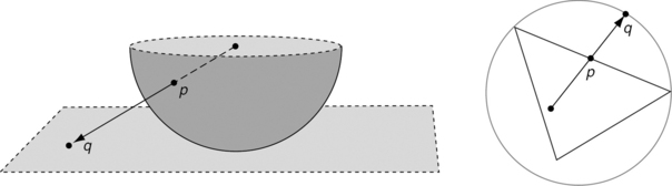
FIGURE 6.12 Left: gnomonic azimuthal projection of an open halfsphere (point p) onto the Euclidean plane (point q). Right: projection of a triangle onto a circle.
A circle with one point removed is homeomorphic to ![]() ; the surface of a sphere with one point removed is homeomorphic to
; the surface of a sphere with one point removed is homeomorphic to ![]() ; and the (hyper)surface of a 4D hypersphere
; and the (hyper)surface of a 4D hypersphere ![]() with one point removed is homeomorphic to
with one point removed is homeomorphic to ![]() . A disk with one point on its frontier removed is homeomorphic to a closed halfplane. A sphere (or cube) with one point on its surface removed is homeomorphic to a closed halfspace of
. A disk with one point on its frontier removed is homeomorphic to a closed halfplane. A sphere (or cube) with one point on its surface removed is homeomorphic to a closed halfspace of ![]() . A disk with two points on its frontier removed is homeomorphic to a closed strip between two parallel straight lines in
. A disk with two points on its frontier removed is homeomorphic to a closed strip between two parallel straight lines in ![]() . A compact subset of
. A compact subset of ![]() can be homeomorphic only to a compact subset of
can be homeomorphic only to a compact subset of ![]() ; this suggests that we should use compact subsets as geometric representations of discrete spaces.
; this suggests that we should use compact subsets as geometric representations of discrete spaces.
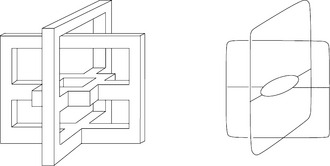
Figure 6.13 (left) illustrates in gray two open squares in the Euclidean plane (each of these squares is homeomorphic to the infinite plane) and, in black, the union of two closed squares that have exactly one point in common (this union is homeomorphic to the union of two disks that “touch” each other at exactly one point, but it is not homeomorphic to the unit disk). Figure 6.13 (right) shows only closed subsets of the Euclidean plane: in gray, two large squares (each homeomorphic to the unit disk) and, in black, the union of two large squares, eight elongated rectangles (representing edges of grid squares), and seven small squares (representing vertices of grid squares); this union is also homeomorphic to the unit disk. Evidently, on the right, we have a geometric representation of two open regions and one closed region of the 2D incidence grid.
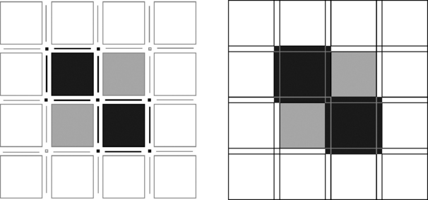
FIGURE 6.13 Left: a disjoint partition of the real plane into open squares (represented by large squares not containing their frontiers), open line segments (not containing their endpoints), and the remaining points (small squares). Right: the geometric representation of subsets of the 2D incidence grid as introduced in Section 2.1.5: a regular tessellation of the plane into (nondisjoint) large closed squares, elongated closed rectangles, and small closed squares, where nondisjoint polygons share an edge or a vertex.
For example, the property of being the empty set is a topologic invariant, and so is the property of being a nonempty set. Dimension (see Definition 6.7) is a nontrivial example of a topologic invariant. Finding topologic invariants is a central problem in topology. Similarly, calculating topologic invariants is a central problem in digital topology. For example, the number of components is a topologic invariant. Poincaré has shown that the Euler characteristic of a regular tessellation of an n-dimensional space is a topologic invariant; we will discuss this result in Section 6.4.5.
Nonhomeomorphy can be proved by comparing topologic invariants; if two sets have different values of a topologic invariant (e.g., different dimensions), they cannot be homeomorphic.
In Figure 6.13 (left), the two gray squares, which are open in ![]() 2, are nonhomeomorphic to the union of the two (closed) black squares. In Figure 6.13 (right), each of the two (closed) gray squares is homeomorphic to the union of the black (closed) squares and rectangles.
2, are nonhomeomorphic to the union of the two (closed) black squares. In Figure 6.13 (right), each of the two (closed) gray squares is homeomorphic to the union of the black (closed) squares and rectangles.
Definition 6.10
Two regions in a 2D (3D) picture are topologically equivalent (homeomorphic) iff their geometric representations in the incidence grid are homeomorphic in ![]() 2 (
2 (![]() 3).
3).
Note that topologic equivalence between picture regions depends on how marginal cells are assigned to principal cells. For example, the two regions of solid dots shown on the left in Figure 6.14 are homeomorphic in the (4,8)-adjacency grid, and their geometric representations in ![]() 2 are homeomorphic to the connected set shown on the right. (As we saw in Section 5.4.1, assuming (4,8)-adjacency is equivalent to assuming ordered adjacency with black > white.) For all of these regions, we have χ = 1. Even if we considered the two regions on the left (incorrectly) as graphs (with v = 48, e = 78, and f = 31 on the left and v = 35, e = 37, and f = 3 on the right, counting all faces equally whether they are holes or atomic cycles), we would obtain χ = + 1 in both cases, because these graphs are planar.
2 are homeomorphic to the connected set shown on the right. (As we saw in Section 5.4.1, assuming (4,8)-adjacency is equivalent to assuming ordered adjacency with black > white.) For all of these regions, we have χ = 1. Even if we considered the two regions on the left (incorrectly) as graphs (with v = 48, e = 78, and f = 31 on the left and v = 35, e = 37, and f = 3 on the right, counting all faces equally whether they are holes or atomic cycles), we would obtain χ = + 1 in both cases, because these graphs are planar.

6.3.2 Isotopy
Two subsets L and M of a topologic space S are called isotopic iff there exists a homeomorphism Φ from S onto itself such that Φ(L) = M.
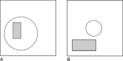
Isotopy is a stronger concept than homeomorphy. For example, suppose S contains a circle C and a rectangle R (see Figure 6.15). In the picture on the left, (A) R is surrounded by C, and, in the picture on the right, (B) R is outside of C. The two pictures are not isotopic in S; there exists no homeomorphism of S onto itself that maps (A) into (B).4
It can be shown that (A) and (B) are isotopic in ![]() 3. The two bands on the left in Figure 6.16 are homeomorphic subsets of
3. The two bands on the left in Figure 6.16 are homeomorphic subsets of ![]() 3, but they are not isotopic in
3, but they are not isotopic in ![]() 3. The two curves γ1 (a meridian) and γ2 (a parallel of latitude) on the surface of the torus shown on the right in Figure 6.16 are isotopic. The curves γ1 and γ3 are isotopic in
3. The two curves γ1 (a meridian) and γ2 (a parallel of latitude) on the surface of the torus shown on the right in Figure 6.16 are isotopic. The curves γ1 and γ3 are isotopic in ![]() 3 but not on the surface of the torus.
3 but not on the surface of the torus.

FIGURE 6.16 Left: two homeomorphic bands; the one below is twisted twice. Right: three curves on a torus.
We can think of regions as being characterized by homeomorphy and pictures as being characterized by isotopy. The following definition makes use of the geometric representations defined in Section 2.1.5.
Definition 6.11
Two 2D (3D) binary pictures are topologically equivalent (isotopic) iff their geometric representations in the incidence grid are isotopic in ![]() 2 (
2 (![]() 3).
3).
As seen in Section 6.3.1, topologic equivalence between pictures depends on how marginal cells are assigned to principal cells. The two binary pictures in the (4,8)-adjacency grid shown in Figure 6.17 can be made isotopic by changing a few pixel values.

FIGURE 6.17 Two nonisotopic binary pictures in the (4,8)-adjacency grid; their rooted region adjacency trees are shown below.
We saw in Theorem 4.2 that a 2D binary picture in the (4,8)- or (8,4)-adjacency grid has a rooted region adjacency tree in which the root represents the infinite background component.
Proposition 6.4
Two 2D binary pictures in the (4,8)- or (8,4)-adjacency grid are isotopic iff they have isomorphic rooted region adjacency trees.
This result generalizes to multivalued 2D pictures. A picture defines a partition of the plane into sets Mu (0 ≤ u ≤ Gmax) in which Mu is the P-equivalence class defined by value u. Two pictures P and P’ (having equivalence classes Mu and ![]() ) are isotopic iff there exists a homeomorphism Φ from
) are isotopic iff there exists a homeomorphism Φ from ![]() 2 into
2 into ![]() 2 such that
2 such that ![]() ) for each u.
) for each u.
6.3.3 Homotopy
Homotopy allows us to give a precise definition of the topologic structure of a region. In particular, it allows us to define “simply connected.”
To define the notion of homotopy, we must first define the fundamental group of a subset M of a topologic space [S, G]. A continuous function ![]() with
with ![]() and
and ![]() defines a parameterized path γ from p to q in M. Two parameterized paths γ1 and γ2 in M that have the same endpoints are called homotopic iff γ1 can be continuously transformed into γ2 in M. More precisely, let the paths γ1 and γ2 be defined by the functions
defines a parameterized path γ from p to q in M. Two parameterized paths γ1 and γ2 in M that have the same endpoints are called homotopic iff γ1 can be continuously transformed into γ2 in M. More precisely, let the paths γ1 and γ2 be defined by the functions ![]() and
and ![]() . A continuous transformation of γ1 into γ2 is a continuous function ψ : [0,1] × [0,1] → M such that
. A continuous transformation of γ1 into γ2 is a continuous function ψ : [0,1] × [0,1] → M such that ![]() and
and ![]() for any real x in [0,1]. If γ2 is a single point,ψ defines a contraction of γ1 in M into a single point.
for any real x in [0,1]. If γ2 is a single point,ψ defines a contraction of γ1 in M into a single point.
Homotopy defines an equivalence relation on the class of all parameterized paths in M. For example, Figure 6.18 shows three paths from p to q in M; γ1 and γ2 are homotopic, but γ3 is not homotopic to γ1 or γ2.

Let p0 ∈ M be the endpoint of γ1 and the starting point of γ2. The product ![]() is defined by concatenation:
is defined by concatenation: ![]() and
and ![]() are combined into a single function
are combined into a single function
This product is compatible with homotopy; if γ1 is homotopic with γ3 and γ2 is homotopic with γ4, then ![]() with
with ![]() .
.
Let [γ] be the class of all paths homotopic in M to γ with respect to a given point p0 of γ. The setπ(M) of all of these classes is a group under ![]() called the fundamental group of M with respect to p0. A path that is contractible in M into the single point p0 is called zero-homotopic. The set of zero-homotopic paths is the identity ε of the groupπ(M) (i.e., for any ξ ∈ Π (M), we have
called the fundamental group of M with respect to p0. A path that is contractible in M into the single point p0 is called zero-homotopic. The set of zero-homotopic paths is the identity ε of the groupπ(M) (i.e., for any ξ ∈ Π (M), we have ![]() ). If the path γ is defined by φ and the path [γ−1] is defined byψ(x) = φ(1 – x), then [γ−1] is the inverse of
). If the path γ is defined by φ and the path [γ−1] is defined byψ(x) = φ(1 – x), then [γ−1] is the inverse of ![]() . Although
. Although ![]() is associative, in general it is not commutative (Abelian).
is associative, in general it is not commutative (Abelian).
If p0 and p1 can be connected by a path in M, the fundamental groups of M with respect to p0 and p1 are isomorphic. It follows that, if M is connected, its fundamental group does not depend on p0. The fundamental group is a topologic invariant in homotopy theory.
This definition is based on work by C. Jordan (1866, on the topologic equivalence of curves) and H. Poincar6 (1892, on the fundamental group).
In other words, M is simply connected iff any parameterized path in M that starts and ends at the same point is contractible in M into a single point. For example, a disk and a ball are both simply connected.
Example 6.3
The fundamental group of a circle is the free cyclic group. A path that goes around the circle clockwise n ≥ 0 times defines a homotopy class αn; a path that goes around the circle counterclockwise m ≥ 0 times defines a homotopy class α−m; the class α0 is the identity ∈. The free cyclic group is isomorphic to the additive group [![]() , +, 0] of the integers and is commutative. A solid torus, an annulus, and the set M shown in Figure 6.18 also have fundamental groups isomorphic to [
, +, 0] of the integers and is commutative. A solid torus, an annulus, and the set M shown in Figure 6.18 also have fundamental groups isomorphic to [![]() , +, 0]. Thus a circle and an annulus are homotopic, but they are not homeomorphic.
, +, 0]. Thus a circle and an annulus are homotopic, but they are not homeomorphic.
The surface of a torus (i.e., a hollow torus) has a fundamental group that contains the identity, the classes of (repeated) “meridians” and (repeated) “parallels” (see Figure 6.16), and the classes defined by products of these classes. This group is commutative, because the product of a meridian cycle followed by a parallel cycle can be homotopically deformed into the product of a parallel cycle followed by a meridian cycle.
As another example, consider two circles that touch at a point p0 and “form figure eight.” The fundamental group of this set is not commutative. The product of a cycle in the upper part followed by a cycle in the lower part cannot be homotopically deformed into the product of a cycle in the lower part followed by a cycle in the upper part
The linear skeleton of a set M ⊆ ![]() n (see Figure 6.19) is defined by continuous contractions; hence a set is homotopic to its linear skeleton.5 For example, the linear skeleton of a simply connected set is a point and that of a torus is a simple closed curve.
n (see Figure 6.19) is defined by continuous contractions; hence a set is homotopic to its linear skeleton.5 For example, the linear skeleton of a simply connected set is a point and that of a torus is a simple closed curve.
6.4 Combinatorial Topology
Combinatorial topology studies partitions of objects into “complexes.” A polyhedron is a finite union of simplexes (in ![]() 3 : points, edges, triangles, or tetrahedra). A digitized subset of
3 : points, edges, triangles, or tetrahedra). A digitized subset of ![]() 2 or
2 or ![]() 3 can be regarded as a partition into convex subsets. A partition into simplexes or convex sets defines a geometric complex. The study of such partitions is of central interest in combinatorial topology.
3 can be regarded as a partition into convex subsets. A partition into simplexes or convex sets defines a geometric complex. The study of such partitions is of central interest in combinatorial topology.
6.4.1 Geometric complexes and the Euler characteristic
An elementary curve γ (to be defined in Chapter 7) can be partitioned into one-dimensional geometric complexes S that consist of arcs (also called 1-cells) and their endpoints (also called isolated points or 0-cells). Let α0 be the number of 0-cells in S and α1 the number of 1-cells in S that contain at least one 0-cell. The difference χ = α0 –α1 is called the Euler characteristic of S. We will see in Section 6.4.5 that any partition of the same elementary curve has the same value of χ.
For example, a circle is partitioned by n ≥ 1 vertices into n arcs; hence χ = 0. For a simple arc with two endpoints, we have x = 1. Figure 6.20 shows the linear skeleton of a tetrahedron, which has α0 = 4 vertices,α1 = 6 arcs, and x = −2. Adding a vertex on any of the arcs increases α0 and α1 by 1 and thus leaves x unchanged.

FIGURE 6.20 (J.B. Listing, 1861) The elementary curve in 3D space (left) is topologically equivalent to both graph representations of a tetrahedron (middle and right).
The connectivity β1 of a one-dimensional geometric complex S is as follows, where β0 is the number of components of S :
β1 is equal to the number of atomic cycles (sets of components with a union that is a simple curve) of S.β0 and β1 are called the first two Betti numbers6 of S. (A general definition of Betti numbers will be given in Section 6.4.5.) Figure 6.21 shows an example with four 0-cells, six 1-cells, two components, and four atomic cycles.

A planar drawing of a one-dimensional geometric complex (see Figure 6.20 [right] and Figure 6.21) can be regarded as a planar-oriented adjacency graph in which we assume clockwise local circular orders at the nodes. This graph has Euler characteristic χ = β0 = α0 –α1 +α2. It follows that β1 = α2 (the number of faces of the graph) is equal to the total number of cycles minus the number of outer cycles, each of which defines the border of a component.
A 2D geometric complex, as introduced by J.B. Listing in 1861, contains a finite number of bounded closed subsets of ![]() 2, which may be faces, curves, arcs, or isolated points (e.g., endpoints of arcs). The complement of the union of all of these compact sets is an open set called the unbounded exterior.
2, which may be faces, curves, arcs, or isolated points (e.g., endpoints of arcs). The complement of the union of all of these compact sets is an open set called the unbounded exterior.
For example, the frontier (surface) of a simple polyhedron in ![]() 3 can be partitioned into elements of a 2D geometric complex called a surface complex of the polyhedron. A single face can be represented by a simple polygon, its edges, and its vertices (the endpoints of the edges). The surface of a simple polyhedron is topologically equivalent to the surface of a sphere. The unbounded exterior of this 2D complex splits into two disjoint open sets (see the separation theorems in Section 7.4), one bounded (the interior of the polyhedron), and the other unbounded. Let α0,α1, and α2 be the number of vertices, edges, and faces of a simple polyhedron. The Descartes-Euler polyhedron theorem (see Equation 4.5)α0 –α1 +α2 = 2 was originally established (by Descartes and Euler) only for convex polyhedra in 3D space, but it is correct for any simple polyhedron.
3 can be partitioned into elements of a 2D geometric complex called a surface complex of the polyhedron. A single face can be represented by a simple polygon, its edges, and its vertices (the endpoints of the edges). The surface of a simple polyhedron is topologically equivalent to the surface of a sphere. The unbounded exterior of this 2D complex splits into two disjoint open sets (see the separation theorems in Section 7.4), one bounded (the interior of the polyhedron), and the other unbounded. Let α0,α1, and α2 be the number of vertices, edges, and faces of a simple polyhedron. The Descartes-Euler polyhedron theorem (see Equation 4.5)α0 –α1 +α2 = 2 was originally established (by Descartes and Euler) only for convex polyhedra in 3D space, but it is correct for any simple polyhedron.
Example 6.4
(M.H.A. Newman, 1939) A rectangular grating (see Figure 6.22) defines a 2D geometric complex. In the grating shown in Figure 6.22, we have α0 = 49 vertices,α1 = 84 edges, and α2 = 36 bounded faces, resulting in χ = 1. The grating is a tessellation of a rectangle into vertices, edges, and rectangles. The sizes and shapes of the cells are unimportant for topologic purposes. Such complexes are of interest for modeling partitions of 2D pictures or of surfaces of 3D objects (see Chapter 11).

In 1813, A. Cauchy generalized the Descartes-Euler polyhedron theorem (see Equation 4.5) by introducing intercellular faces into the polyhedron. This results in the following,
where α3 is the number of polyhedral cells; see Figure 6.23 (left). Cauchy considered only convex polyhedra.

FIGURE 6.23 Left: a cube partitioned into eight subcubes has α0 = 27 vertices,α1 = 54 edges,α2 = 36 faces, and α3 = 8 subpolyhedra. Right: a parallelepiped with b = 3 cube-shaped bubbles, t = 2 tunnels, and p = 4 polygons on its faces; here α0 = 48,α1 = 72, and α2 = 32.
In 1812, A.-J. Lhuilier suggested a generalization that also allowed “tunnels” and “bubbles.” He claimed that the following was true,
where b is the number of bubbles, t the number of tunnels, and p the number of polygons (“exits of tunnels”) on faces of the polyhedron. His discussion of the number of tunnels did not cover the full range of possibilities. For example, Figure 6.19 illustrates the difficulty of defining a tunnel; in fact, an object such as a sponge can have a “network” of tunnels. Numbers of cavities (bubbles) and tunnels will be discussed further in Section 6.4.5.
3D geometric complexes are used to model partitions of 3D sets into convex polyhedra or simplexes. A partition must be “complete” (e.g., if a polyhedron is in the complex, its surface complex must also be in the complex). The object in Figure 6.19 is a 3D geometric complex that has α0 = 88 vertices,α1 = 132 edges,α2 = 36 faces (assuming a straightforward partition of the surface into a surface complex), and one solid cell (α3 = 1). The Euler characteristic of the 2D surface complex is χ = α0 –α1 +α2 = −8 (regarding the object as a hollow surface), and that of the 3D object is χ = α0 –α1 +α2 –α3 = −9.
6.4.2 Euclidean complexes
The geometric complexes discussed so far are Euclidean complexes, which are partitions into compact convex sets. As a default, we assume that these sets are convex polyhedra. Surface complexes will be defined in Chapter 7.
The notion of dimension plays an important role in the definition of complexes. Dimension allows us to distinguish isolated points from line (or arc) segments and edges from faces. (In a vector space, the dimension of a set is the greatest number of linearly independent vectors in the set, but this is not a topologic characterization.)
Let C ⊂ ![]() n be a convex polyhedron and let P be an m-dimensional subspace (m <n) of
n be a convex polyhedron and let P be an m-dimensional subspace (m <n) of ![]() n. P ∩ C is called an (n − 1)-side of C if dim(P ∩ C) = n − 1. A nonempty intersection of finitely many (n − 1)-sides is called a proper side; if it has dimension k, it is called a k-side. Every (n − 2)-side is a side of exactly two (n − 1)-sides. The 0-sides of C are its vertices. C is an improper side of itself. If C is bounded, it is called a convex cell.
n. P ∩ C is called an (n − 1)-side of C if dim(P ∩ C) = n − 1. A nonempty intersection of finitely many (n − 1)-sides is called a proper side; if it has dimension k, it is called a k-side. Every (n − 2)-side is a side of exactly two (n − 1)-sides. The 0-sides of C are its vertices. C is an improper side of itself. If C is bounded, it is called a convex cell.
Let M ⊆ ![]() n be the union of a finite number of convex cells. A Euclidean complex is a partition S of M into a nonempty finite set of convex cells that has the following properties:
n be the union of a finite number of convex cells. A Euclidean complex is a partition S of M into a nonempty finite set of convex cells that has the following properties:
E1: If p is a cell of S and q is a side of p, then q is a cell of S.
E2: The intersection of two cells of S is either empty or a side of both cells.
The union of the cells of S need not be connected, and a subset of the cells of S need not define a Euclidean complex.
Figure 6.24 shows four partitions of a (nonsimply connected) polygon. For the partition into squares on the left, we have α0 = 106,α1 = 165, and α2 = 59 (not counting the hole); for the partition into triangles on the right, we have α0 = 106,α1 = 224, and α2 = 118. Both counts result in x = 0. Grid cell complexes formed by cells in ![]() are examples of Euclidean complexes. The partition on the left in Figure 6.24 is a 2D grid cell complex, and the partition on the right is a triangulation (see Section 6.4.3). For the partitions in the middle (where we also count the hole as a face), we have α0 = 59,α1 = 76, and α2 = 18 and α0 = 61,α1 = 79, and α2 = 19 so that χ = 1.
are examples of Euclidean complexes. The partition on the left in Figure 6.24 is a 2D grid cell complex, and the partition on the right is a triangulation (see Section 6.4.3). For the partitions in the middle (where we also count the hole as a face), we have α0 = 59,α1 = 76, and α2 = 18 and α0 = 61,α1 = 79, and α2 = 19 so that χ = 1.
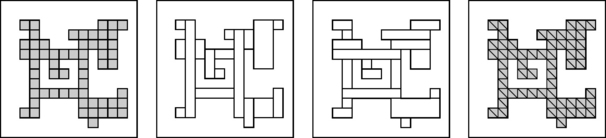
FIGURE 6.24 Four partitions of a polygon. The two in the middle require vertices at the branching points to become Euclidean complexes that satisfy E2.
Figure 6.25 shows the 1-component illustrated in Figure 6.24 (in the grid point model), as well as another 1-component. The 1-component on the left has 12 atomic cycles, one inner border cycle, and one outer border cycle (i.e.,α2 = 14,α1 = 71, and α0 = 59) so that x = α0 − α1 + (α2 − 1) = 1. The single inner border cycle defines a hole; it is not counted in the Euler characteristic of the Euclidean complex, so χ = 0 for the complex. The second 1-component has the same values of χ (0 for the Euclidean complex and 1 for the oriented adjacency graph); the two 1-components are homeomorphic (see Definition 6.10). Note that the adjacency graphs of the components are different; the graph of the component on the left is not 2-strong, but the graph of the other component is 2-strong.

FIGURE 6.25 From left to right: the 1-component (shown in Figure 6.24) in the grid point model; a sketch of the contributing grid points, with edges representing adjacencies, and atomic cycles; another 1-component; its grid point representation.
6.4.3 Simplicial complexes; triangulations
A Euclidean complex is called simplicial iff all of its cells are simplexes. An n-dimensional simplex (n-simplex) is the convex hull of n + 1 vertices p0, p1,…, pn, where the vectors ![]() are linearly independent. For example, a 3-simplex is a solid tetrahedron. Complexes with cells that are tetrahedra are of special interest for modeling the boundaries of 3D isothetic grid polyhedra [476].
are linearly independent. For example, a 3-simplex is a solid tetrahedron. Complexes with cells that are tetrahedra are of special interest for modeling the boundaries of 3D isothetic grid polyhedra [476].
A finite Euclidean complex that contains only triangles, line segments, and points is called a triangulation; evidently, such a complex is simplicial. The frontier of any polyhedron can be triangulated.
Figure 6.26 shows three examples of triangulations. We will now illustrate how polyhedral surfaces can be constructed by identifying vertices in the triangulation on the right. If we identify P5, P8, P11, and P14 (the four corners of the large square), the (directed) line segment P5P14 becomes identified with (“glued to”) the directed line segment P8P11, as does P5P8 with P14P11. If we then identify P6 with P13, P7 with P12, P9 with P16, and P10 with P15, it can be shown that the resulting triangulation is homeomorphic to the surface of a torus. If instead we identify P6 with P12, P7 with P13, P9 with P16, and P10 with P15, the resulting triangulation is homeomorphic to a Klein bottle.

FIGURE 6.26 (P.S. Aleksandrov, 1956) A planar triangulation (left), a polyhedral surface homeomorphic to the surface of a torus (middle), and a triangulated rectangle (right; see text for details).
If we identify vertices P1,P2,P3, P4, P17, P18, and P19; P5 and P11; P6 and P12; P7 and P13; P8 and P14; P9 and P15; and P10 and P16, we have a triangulation of the projective plane (P.S. Aleksandrov, 1956). These examples can serve as a warning not to underestimate the complexity of triangulations, even if they have small cardinalities. A triangulation used in a surface analysis algorithm (in 3D picture analysis) should certainly not contain a Klein bottle or a projective plane!
Any polyhedral surface is compact. The frontier of a simple polygon (as defined in Section 1.2.2) is an example of the union of a one-dimensional triangulation; it too can be regarded as a polyhedral surface.
The dimension of a triangulation is the maximum dimension of its elements. A 2D triangulation T is called pure iff every point or line segment in T precedes some triangle in T with respect to the side-of relation. The surface of a simple polyhedron is the union of a pure 2D triangulation.
A path of sets(M1,M2,…,Mn) is a finite sequence of sets such that Mi ∩ Mi+1 1 ≠ø (i = 1,…, n−1). Such a path connects M1 with Mn. A polygonal path is a path of line segments. A pure 2D triangulation T is called strongly connected iff every two triangles T1 and T2 in T are connected by a path of triangles, all of which are in T. The surface of a simple polyhedron is a strongly connected triangulation. The analysis of simple polygons and simple polyhedra is often done with the aid of triangulations.
6.4.4 Abstract complexes
The theory of finite abstract complexes is based on a partial ordering that generalizes a reflexive, transitive, antisymmetric “bounded-by” relation rather than the reflexive, symmetric, and in general nontransitive incidence relation.
Let S be a finite or countably infinite set of points. Assign a nonnegative integer dim(c), which is called the dimension of c, to each c ∈ S. The following definition goes back to the axiomatic definition of geometric complexes by E. Steinitz in 1908 and to the topologic study of abstract complexes by A.W. Tucker in 1933. An abstract complex [S, ≤, dim] has two properties:
An abstract complex is an example of a poset topology. The elements of S are called the cells of the complex. The study of abstract complexes does not depend on interpreting cells as vertices, edges, faces, and so forth. Any subset of an abstract complex is also an abstract complex and defines a topologic subspace of the complex.
If dim(c) = i, we call c an i-cell. The index dimension of an abstract complex is n iff dim(c) ≤ n for all c ∈ S and dim(c) = n for at least one c ∈ S.
The “side-of” relation in a Euclidean complex is an example of the relation ≤ and has property C2. If c1 ≤ c2 and c1 ≠ c2, we say that c1 is a proper side of c2. Two cells are incident iff c1 ≤ c2 or c2 ≤ c1.
Let [S,I, dim] be an incidence pseudograph. We say that c < c’ if c′ ∈ I(c), c ≠ c′, and dim(c) < dim(c′). If we define c ≤ c′ iff c < c′ or c = c′, [S, ≤, dim] is an abstract complex. Thus our discussion about incidence pseudographs in Chapter 5 can be translated into a language of abstract complexes.
6.4.5 The Poincaré formula
We conclude this chapter with a brief treatment of homology theory. Polyhedra are characterized in combinatorial topology by homology (which is easier to define than homotopy), homology groups, and Betti numbers. The Poincaré formula7 describes the Euler characteristic of a partition of a polyhedron (a complex) by its Betti numbers. This provides a general proof that Euler characteristics are topologic invariants. A precise statement of the Poincaré formula requires a brief introduction to homology theory.
Let [S, ≤, dim] be a Euclidean complex. We write c ∈ S as c(i) if dim(c) = i. In Section 5.2.1, we defined i-chains in S as expressions of the form ![]() where bk = 0 or 1, and the sum is over all i-dimensional cells in S. We recall that i-chains can be added modulo 2. We say that
where bk = 0 or 1, and the sum is over all i-dimensional cells in S. We recall that i-chains can be added modulo 2. We say that ![]() is in C(i) iff bk = 1, and we write C(i) = 0 if every bk is 0. Let ∪ C(i) be the union of the cells in C(i). Evidently, C(i) = 0 iff ∪ C(0) = φ.
is in C(i) iff bk = 1, and we write C(i) = 0 if every bk is 0. Let ∪ C(i) be the union of the cells in C(i). Evidently, C(i) = 0 iff ∪ C(0) = φ.
In Section 5.2.1, we defined the frontier ![]() of an i-chain
of an i-chain ![]() , and, if i> 0,
, and, if i> 0, ![]() is the (i − 1)-chain
is the (i − 1)-chain ![]() where ak is the number of i-cells in C(i) that are incident with
where ak is the number of i-cells in C(i) that are incident with ![]() . C(i) is called an i-cycle if
. C(i) is called an i-cycle if ![]() . Any 0-chain is a 0-cycle, and the frontier of any chain is a cycle, because
. Any 0-chain is a 0-cycle, and the frontier of any chain is a cycle, because ![]() .
.
We write the following if there is an i-chain C(i) such that ![]() C(i−1) ∼0
C(i−1) ∼0
We write C(i) ∼ C′(i) iff C(i) + C′(i) ∼ 0. Evidently, ∼ is an equivalence relation; it is called a homology.
Let K =[S, ≤, dim] be a Euclidean complex with index dimension n. A set B of i-cycles of k is called a basis for the i-cycles of K with respect to homology if every i-cycle C(i) of K is homologous to a sum of i-cycles of B; in essence, there are coefficients ak such that the following imply bk = 0 (modulo 2) for all k:
The cardinality βi of a basis for the cycles of K is called the ith Betti number of K.
This theorem was originally proved by H. Poincaré only for n = 2 (i.e., for 2D manifolds [surfaces] in 3D Euclidean space).
The Euler characteristic is defined by the following where αi is the number of i-cells in K:
Theorem 6.8 through 6.9 imply the following:
Proposition 6.5
The Euler characteristic of a Euclidean complex is a topologic invariant.
Example 6.5
If K is the surface of a sphere, we have β0 = 1, β1 = 0, and β2 = 1 so that χ = 2. For the surface of a torus, we have β0 = 1,β1 = 2, and β2 = 1 so that χ = 0. If K is a sphere with n ≥ 1 handles (informally, tori) attached to it, we have β0 = 1,β1 = 2n, and β2 = 1 so that χ = 2 − 2n. These three examples are illustrated in Figure 6.27 on the right. For any closed surface, we have β0 = 1 and β2 = 1; hence closed surfaces differ only in β1, which is even for orientable surfaces and odd for nonorientable surfaces. For a solid sphere, we have β0 = 1,β1 = 0, and β2 = 0 so that χ = 1. If the solid sphere has n ≤ 1 (pairwise nonconnected) cavities so that it has n + 1 closed orientable surfaces, we have β0 = 1,β1 = 0, and β2 = n so that χ = hbox1 − n. Three solids are illustrated in Figure 6.27 on the left.
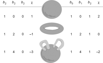
Let K be a bounded 3D set that consists of several connected components and with a surface that consists of several orientable closed surfaces. For this K, β0 is the number of connected components,β1/2 is the number of tunnels, and β0 +β2 is the number of closed surfaces (so that there are β2 cavities).
Let K be the edge skeleton (a one-dimensional complex) of a tetrahedron; it has v = 4 vertices, e = 6 edges, and f = 0s faces. Here we have β0 = 1,β1 = 3 (note that the 1-cycle around each triangle is the sum of the three 1-cycles around the other three triangles), and β2 = 0 so that χ = −2. Note that we do not have “1.5 tunnels” in this case; the edge skeleton is not a surface. For one-dimensional complexes in 3D space,β0 is the number of components, and β1 is the number of tunnels. A one-dimensional complex in the plane has β1 holes (the 2D analog of tunnels). Note that a Euclidean one-dimensional complex is always a planar graph (i.e., faces are not counted in its Euler characteristic, because it is only one-dimensional), and β1 is its number of internal faces, excluding the unbounded external face; see Figure 6.28. Oriented adjacency graphs allow us to generalize the Euler characteristic and not be limited to planar graphs. See Section 17.5 about tunnel-free subsets of Gm,n,l.

FIGURE 6.28 Left: a 2D incidence grid representation of a closed region in a 2D picture with α0 = 106,α1 = 165,α2 = 59,β0 = 1,β1 = 1, and β2 = 0 so that χ = 0. Middle: the same region in the oriented 4-adjacency graph with α0 = 59,α1 = 71,α2 = 14,β0 = 1,β1 = hbox1, and β2 = 0 so that χ + = χ + 1 = 1. Right: a planar one-dimensional complex (note: no faces) with α0 = 59,α1 = 71,β0 = 1, and β1 = 13 so that χ = −12.
6.4.6 Homology groups
Betti numbers can also be defined using homology groups. Let [G, +, 0] be an additive abelian group with identity 0. [H, +, 0] is called a subgroup of [G, +, 0] iff H ⊆ G and f,g ∈ H imply f – g ∈ H. A homomorphism φ from [G, +, 0] onto [H, +, 0] is a function from G onto H such that φ(f) –φ(g) = φ(f – g) for all f, g ∈ G. If φ is one-to-one, it is called an isomorphism. If φ is a homomorphism, H = φ−1(0) is a subgroup of G called the kernel of φ. The kernel of an isomorphism is the singleton {0}.
Let H be a subgroup of G and f ∈G. fH = {f + g : g ∈ H} is called a coset of G relative to H. Note that two cosets are either disjoint or identical. The set of cosets of G relative to H is an additive group called the factor group G/H of G modulo H; we define fH + gH = (f + g)H.φ : G → G/H is a homomorphism and H is its kernel.
The set C(i) of i-chains of a Euclidean complex K is an abelian group under addition modulo 2. Let G(i) be the subgroup of C(i) that consists of all i-cycles, and let F(i) be the subgroup of G(ii) that consists of all frontiers ϑC(i+1) of (i + 1)-chains. The factor group H(i)= G(i)/F(i) is called the i-th homology group (Betti group) of K. The homology ∼ partitions the cycles G(i) into equivalence classes called homology classes. It can be shown that the dimension of H(i) is the i-th Betti number.
Example 6.3 showed that the surface of a torus and a planar drawing of an 8 have different fundamental groups (i.e., they are not identical with respect to homotopy). On the other hand, the homology groups of both of these sets are isomorphic to the direct sum [![]() , +, 0]
, +, 0] ![]() [
[![]() , +, 0]. Thus isomorphism of homology groups does not imply homotopy (isomorphism of fundamental groups).
, +, 0]. Thus isomorphism of homology groups does not imply homotopy (isomorphism of fundamental groups).
6.5 Exercises
1. Does the adjacency grid ![]() have a topology in which 1-connectedness is the same as topologic connectedness?
have a topology in which 1-connectedness is the same as topologic connectedness?
2. Describe the Aleksandrov topology of the poset [![]() , ≤].
, ≤].
3. Explain why the product of one one-dimensional grid cell topology and two one-dimensional grid point topologies is already contained in the set of 3D digital topologies listed after Theorem 6.6.
4. Show that the Euler characteristic χ(Π) of a polyhedron Π ⊂ ![]() 3 can also be defined by the following axioms:
3 can also be defined by the following axioms:
2. χ(Π) = 1if Π is nonempty and convex.
3. If Π1 and Π2 are polyhedra,χ(Π1 ∪ Π2) = χ(Π) +χ(Π2) –χ(Π1 ∩ Π2).
(Hint: Prove that χ(Π) is equal to the alternating sum α0 –α1 +α2 where α0 is the number of vertices,α1 the number of edges, and α2 the number of triangles in any triangulation of Π’s frontier.)
5. Prove that, for any (planar) polyhedron Π ⊂ ![]() 2,χ(Π) is equal to the number of components of Π (in the Euclidean topology) minus the number of holes in Π.
2,χ(Π) is equal to the number of components of Π (in the Euclidean topology) minus the number of holes in Π.
6. Let ni be the number of 2× 2 patterns of pixels in a binary picture P that contain exactly i 1s (i = 0,1,2,3,4), and let nD be the number of such patterns that contain two diagonally adjacent 1s. Let the following be true:
E8,4(P) = (n1 – n3 – 2nD)/4 and E4,8(P) = (n1 – n3 + 2nD)/4
The geometric realization of the 2D grid cell topology based on the label order “0 < 1” or “1 < 0” maps the union of the 1s in P into a (planar) polyhedron Π. Prove that χ(Π) = E8,4(P) for label order “0 < 1” and that χ(Π) = E4,8(P) for label order “1 < 0” (see Figure 17.2 for an example).
7. Prove that any convex set in ![]() n (e.g., a single point, a straight line segment, a sphere, a convex polyhedron) is simply connected (i.e., its fundamental group is {ε }).
n (e.g., a single point, a straight line segment, a sphere, a convex polyhedron) is simply connected (i.e., its fundamental group is {ε }).
8. Prove that the free cyclic group is the fundamental group of the annulus and also of ![]() 2/{p}, where p is any point in
2/{p}, where p is any point in ![]() 2.
2.
9. Prove that α0 –α1 = 1 for any tree (i.e., that the Euler characteristic of any tree is 1).
10. We have given finite and countable examples of abstract complexes. The following is a noncountable example: Let S = {sa : a ∈ [0,1]} be a noncountable set of abstract cells defined on the real index interval [0,1], where sa ≠ sb iff a ≠ b. For a ∈ [0,1], let a = 0 and a1a2a3 … where ai∈ {0,1,…,9}. Let sa ≤ sb iff a = b or a1 < b1 and ai = bi for all i ≥ 11. Let dim(sa) = a1. Show that [S, ≤, dim] is an abstract complex.
11. Calculate the Betti numbers of the following three tilings (2D complexes):

12. Suppose deletion of all of the invalid edges in a picture leads to the nonconnected undirected graph shown below. Regard each pixel as the centroid of an isothetic unit square, and take the union of all of the squares that correspond to pixels in the same 4-component. The frontiers of the resulting sets are isothetic simple curves. Find the Betti numbers βi of these sets (i = 0,1,2).

13. Calculate the number of tunnels in the one-dimensional complex that consists of the vertices and edges of a tetrahedron.
14. Consider three “systems of pathways” in a solid sphere: (1) n ≥ 3 straight pathways that start at the surface of the sphere and meet at its center; (2) four pathways that form a hollow tetrahedron inside the sphere, with an exit to the surface of the sphere, at each vertex of the tetrahedron; and (3) a pathway that forms a hollow torus inside the sphere, with n ≥ 1 exits to the surface of the sphere. What are the numbers of tunnels in these three cases?
15. The Arens-Fort space is defined on the (countable) set S = ![]() 2 by a set G that is the union of
2 by a set G that is the union of ![]() 2/{(0,0)} and the family of all sets U ⊂
2/{(0,0)} and the family of all sets U ⊂ ![]() 2 with projections {n :(m, n) ∈ U} that are finite for all but finitely many m ∈ n. Show that [S, G] is a topologic space and does not have a countable basis.
2 with projections {n :(m, n) ∈ U} that are finite for all but finitely many m ∈ n. Show that [S, G] is a topologic space and does not have a countable basis.
16. Let M ⊆ ![]() be closed iff either 1 ∈ M or ∑n∈M1/n is finite (note that this excludes 0 ∈ M). Show that this defines a topologic space on n that does not have a countable basis for the neighborhoods of 1.
be closed iff either 1 ∈ M or ∑n∈M1/n is finite (note that this excludes 0 ∈ M). Show that this defines a topologic space on n that does not have a countable basis for the neighborhoods of 1.
6.6 Commented Bibliography
There are many textbooks about topology and, in particular, combinatorial topology; see, for example, [9,10,13,100,112,639,771,844,857]. [580] is an edited book about digital topology.
Research regarding topologic approaches to picture analysis began before 1970. In 1966 and 1970, A. Rosenfeld initiated the study of connected subsets of the grid [881, 921]. The relevance of Definition 6.7 to picture analysis was discussed in 1971 by J. Mylopoulos and T. Pavlidis [756]. Figure 7.4 is from [100]. The grid point topology (Section 6.2.2) was described in [1140].
Axiomatic digital topology (axioms for connectedness) was studied in [970]; [872] extended this work. Properties D1 and D2 are due to U. Eckhardt and L. Latecki [297]. Property D3 was added by Y. Kong (private communication, March 2003); see also his discussion of digital topologies in [570]. Digital topology on graphs is studied in [124, 158, 780]; see also [6] and [925]. Theorem 6.4 is proved in [172]; see also [620]. Introductory and review papers about digital topology include [571, 572, 576, 577, 579, 581, 891, 893]; see also [136]. For the relationship between continuous and digital topology, see [95]. For “well-composed” pictures for which 4- and 8-connectedness are equivalent, see [621, 622, 625].
The two-volume book by P.S. Aleksandrov [9, 10] provides a broad coverage of Euclidean and abstract complexes. For more about abstract complexes, see also [1025] and [1069]. For topologies on such complexes, see for example, [9, 844, 1069]. Geometric complexes were introduced into the mathematical literature by J.B. Listing in 1861; see also Section 1.2.6. For Theorem 6.8, see [12]. [999] introduced cellular complexes into the picture analysis literature. See [116] about oriented simplicial complexes and about the encoding of finite subsets of such complexes.
For the topology of polyhedra, see the monographs [709, 844, 1026]. Exercises 4 and 5 are discussed in [577]. See [631] about counting tunnels by counting nonseparating cuts, which gives β1. For the difficulty of defining tunnels for polyhedra in ![]() 3, see [575]. A polygonal loop in
3, see [575]. A polygonal loop in ![]() 3 that is not contractible to a point in the complement of a polyhedron Π obviously defines one tunnel in Π. However, as indicated in Section 6.4.5, there exist dependencies between such loops, and we can only define numbers of tunnels (see also Exercise 14).
3 that is not contractible to a point in the complement of a polyhedron Π obviously defines one tunnel in Π. However, as indicated in Section 6.4.5, there exist dependencies between such loops, and we can only define numbers of tunnels (see also Exercise 14).
Exercise 6 follows [377]. Calculations of Euler characteristics based on local pattern counts in 2D or 3D pictures are reviewed in [577]. For other references about the calculation of the Euler characteristic, see [88, 186, 266, 646, 938]. Local patterns in binary pictures can also be used to provide more detailed topologic classifications of components [14].
Fundamental groups of digital pictures are discussed in [567, 692]. Effective methods of computing presentations of fundamental groups of arbitrary polyhedra are described in [709]. The problem of determining whether two polyhedra have isomorphic fundamental groups is undecidable. (For any finite group G, one can construct a polyhedron with a fundamental group that is isomorphic to G [see Theorem 3.3.20 in [709]], and isomorphism of finite groups is undecidable.) However, the restriction of polyhedra to subsets of ![]() 3 may define a “simpler” subproblem, and a decision algorithm for this subproblem could be used to determine whether a polygonal loop in
3 may define a “simpler” subproblem, and a decision algorithm for this subproblem could be used to determine whether a polygonal loop in ![]() 3 is knotted by determining whether the complement of the loop has the trivial fundamental group. An algorithm for the homotopy classification of binary pictures is given in [158]. Homotopy in digital spaces is studied in [54]. Topologic equivalence, which is called “component equivalence” and defined as a counterpart of homeomorphism for quantized spaces, was discussed in [757]. Topologic equivalence between preimages and “continuous analogs” of digitized sets—and its dependency on the grid constant—is studied in [624].
3 is knotted by determining whether the complement of the loop has the trivial fundamental group. An algorithm for the homotopy classification of binary pictures is given in [158]. Homotopy in digital spaces is studied in [54]. Topologic equivalence, which is called “component equivalence” and defined as a counterpart of homeomorphism for quantized spaces, was discussed in [757]. Topologic equivalence between preimages and “continuous analogs” of digitized sets—and its dependency on the grid constant—is studied in [624].
For Exercise 15, see [1016].
1Also spelled Alexandroff.
2For completeness, we mention that S is called a T1-space iff, for any two distinct points of S, each of the points has a neighborhood that does not contain the other. S is called a T2-space or Hausdorff space iff any two distinct points of S have disjoint neighborhoods. For example, Euclidean space is a Hausdorff space.
3Following [577], these geometric realizations could also be called continuous analogs. We prefer to avoid the term “continuous” for geometric realizations that are defined by discrete sets.
4A formal proof of this can be given on the basis of the local dimensionalities of points in S; for the necessary concepts, see Section 7.1.2.
5In 1861, J.B. Listing introduced the linear skeleton under the name cyclomatic diagram. Because the term “skeleton” has become popular in picture analysis in the context of distance transforms, thinning operations, and so forth (see Sections 3.4.2 and 16.3), it may be preferable to use Listing’s original term “cyclomatic diagram” instead of “linear skeleton.”
6The Italian mathematician E. Betti (1823−1892) published, in 1871, a memoir that defined Betti numbers. Betti’s work inspired H. Poincaré to study topology; Poincaré introduced the term “Betti numbers.”
7This is often called the “Euler-Poincaré formula” but in fact is entirely due to H. Poincaré; it is inspired by the Euler-Descartes theorem about polyhedra.