
Transformations
Subfields of geometry are sometimes defined by systems of axioms and sometimes by groups of transformations under which certain geometric properties remain invariant. This chapter describes the transformation-based approach and presents a set of axioms for digital geometry. It discusses transformation groups and symmetries, neighborhood-preserving transformations, applying transformations to pictures, magnification and demagnification, and digital tomography.
14.1 Geometries
A wide variety of geometries have been developed, motivated by a wide variety of applications: Euclidean (Thales of Miletus, Hippocrates of Chios, the secret society of the Pythagoreans, Euclid, Archimedes); analytic (Descartes, also known as Cartesius); perspective (Alberti, da Vinci, della Francesca, Dürer); projective (Desargues, Pascal); descriptive (Monge); non-Euclidean, such as elliptic and hyperbolic (Lobachevsky, Bólyai, Riemann); and combinatorial (Helly, Borsuk, Erdõs).
The Norwegian mathematician S. Lie and the German mathematician F. Klein formulated a classification system for all of the geometries known at their time:
Geometric properties of objects are those which are invariant with respect to a specified group of transformations.
This classification scheme is known as the 1872 Erlangener Programm of F. Klein. Let B be a base set and G a group of transformations defined on B. The theory of invariants with respect to B and G, which studies quantities that can be measured in B that have values that are invariant under the transformations in G, defines a geometry in which a nonempty family of subsets (“objects” or “figures”) F⊆ ℘(B) is specified as the class of objects of interest. We assume that these objects and the quantities (“properties”) that are measured for them are in fact of practical or theoretic interest.
For example, B might be the 3D Euclidean space E3 = [R3, de] defined by the manifold R3 of triples of real numbers and the Euclidean metric de; F might be the family of all bounded polyhedra; and G might be the group of (i) all similarity transformations, (ii) all affine transformations, or (iii) all projective transformations of B into the Euclidean plane. This defines three different geometries of polyhedra in the sense of the Erlangener Programm.
The study of invariants also requires some relationship among the elements of B (i.e., B must have a structure defined by a metric [see Chapter 3] or a topology [see Chapter 6]). For example, for the invariance of cross-ratios in projective geometry, we make use of the Euclidean metric; for the invariance of simple connectedness, we usually make use of the Euclidean topology.
If at least one of B, G,or F is finite or discrete, the geometry is called a discrete geometry. A set A ⊆ B is called discrete in B iff any p ∈ B has a neighborhood U (p) ⊆ B such that U (p) ∩ A is finite. For example, any set of grid points is discrete in Rn. A family of sets G ⊆ ℘(B) is discrete in B iff any p ∈ B has a neighborhood U (p) ⊆ B that has nonempty intersections with only a finite number of the sets in G. For example, any set of cells of a Euclidean complex (see Section 6.4.2) is discrete in Rn.
Digital geometry, using either the grid point or grid cell model, is a discrete geometry. The structure in the base set B of a discrete geometry is specified by (at least) a system of algebraic neighborhoods U (p) ⊆ B for all p ∈ B, where U is reflexive, symmetric, and nontransitive. An element q is a proper neighbor of p (adjacent to p) iff q ∈ U(p) and p ≠ q. Adjacency structures [S,A] (see Chapter 4) allow us to introduce such neighborhoods; q ∈ U(p) iff p = q or q ∈ A(p).
Packings, tessellations, polyhedra, and Euclidean complexes all involve discrete families of sets in Euclidean space. Geometry on graphs and finite geometries are other examples of discrete geometries. Some of them can be regarded as generalizations of digital geometry if their base set B has an adjacency grid or incidence grid (or cell complex) as an interpretation (i.e., as a model in the sense of logic).
14.2 Axiomatic Digital Geometry
Many geometries can be defined by systems of axioms. Eukleides (also known as Euclid; see Section 1.2.2) also formulated in 13 books an axiom system for the geometry known today as Euclidean geometry. Such a system should be complete, nonredundant, and consistent [384].1 This book has introduced theories based on axioms (e.g., the theory of oriented adjacency graphs based on properties A1 through A4). Consistency is ensured by the existence of nontrivial models.
At the end of the 19th century, there were still many open problems related to the axiomatic foundations of geometries. Poincaré, Pasch, and Hilbert were among those who studied such problems. At the end of the 19th century, mathematicians recognized that Euclid’s axiom system was incomplete. For example, Euclid did not define precise concepts of “between,” “inside,” or “outside”; his reasoning about these concepts was based on pictures. In 1899, D. Hilbert [436] proposed a modified axiom system for Euclidean geometry that removed some of these defects. His work and the work of H.G. Forder [334] formalized Euclidean geometry and proved the consistency of its axioms.
Removing redundancy from a set of axioms system is not critical (in principle), but constructing a complete and consistent set of axioms is. K. Gödel [363] proved that no set of axioms can be both consistent and complete (Gödel’s Incompleteness Theorem). It follows that a consistent set of axioms cannot be complete.
The following axiomatic definition of digital geometry (based on an adaptation of a subset of Hilbert’s axiom system) was presented in a 1989 habilitation thesis [449] by A. Hübler.
Let B be a set of points and G⊆ ℘(B) a nonempty set of lines. We begin with two incidence axioms:
G1: For any two distinct points p,q ∈ B, exactly one line in G contains p and q.
G2: For any line γ ∈ G, there exist pairwise distinct points p,q,r ∈ B such that p ∈γ and q ∈γ but r ∉![]() γ.
γ.
According to axiom G2, there are at least three points in B. Using axiom G1, it then follows that there are at least three pairwise distinct lines in G. It also follows that any two distinct lines can have at most one point in common. (As we saw in Figure 7.11, “crossings” of lines that have no common point are also possible.)
Let || be a relation of parallelism on G that satisfies the following:
G3: || is an equivalence relation on G, and, for any line γ ∈G and any point p ∈ B, there is exactly one line γ′ such that p ∈γ′ and γ ||γ′.
The equivalence relation || defines equivalence classes in G that are called directions.
Let γ(p, q) be the line uniquely defined by points p and q (see axiom G1). A one-to-one mapping Φ from B onto B is called a translation on B iff it is either the identity mapping I or it has the following three properties:
The following axiom guarantees that there are translations that are different from I:
From this and the previous axioms, it follows that there is exactly one translation Φ such that Φ(p) = q.
A translation Φ ≠ I is called cyclic iff there is an integer n> 0 such that Φn(p)= p for all p ∈ B. A translation is cyclic iff Φn(p)= p for some n> 0 and some p ∈ B. The smallest such integer is called the cycle of Φ. [449] shows that, if there exists a cyclic translation with cycle m> 0, all translations in T that are different from I are also cyclic with the same cycle m, and m is a prime number. [449] provided models of axioms G1 through G4 with cyclic translations, for finite or countable infinite sets of points B. Nonparallel lines need not intersect.
Next we introduce axioms of order. Let < and > be two opposite total orders on a line γ (i.e., for all p, q ∈γ, we have p <q iff q> p). Let [γ, <] and [γ, >] denote these oriented lines. Let B ⊆ B3 be the betweenness relation on B for any three pairwise distinct points p, q, r on [γ, <]:
(Possibly this axiom already excludes models with cyclic translations; see the statement following G7.) It follows that any line contains (countably) infinitely many points. Axioms G1 through G5 no longer have finite models.
The following axiom excludes nondiscrete models such as Euclidean geometry:
This requires lines to be countable and isomorphic (with respect to the order) to [Z, <]. Oriented lines can be identified with ordered point sequences {pi}i∈Z.
G7: Let γ1,γ2, and γ3 be three pairwise distinct parallel lines. Let γ and γ′ be two lines that intersect γ1,γ2, and γ3, and let {pi} = γ ∩γi and {p′i} = γ′ ∩ γi (i = 1,2,3). Then B(p1,p2,p3) iff B(p′1,p′2,p′3).
This axiom implies that B(p,q,r) implies B(Φ(p), Φ(q),Φ(r)) for any translation Φ. It also follows [449] that a model of axioms G1 through G7 cannot have a cyclic translation.
For any line γ and any point p ∈γ, there is a translation Φ such that γ = {Φi(p): i ∈ Z}. Such a translation Φ is called a generator of γ. If Φ is a generator of γ, so is Φ−1. Any line γ has exactly two generators, and two lines are parallel iff they have the same generators.
A translation Φ is called atomic iff there is no translation Ψ such that Φ = Ψn and n ≠ 1. A translation is atomic iff it is a generator of a line.
S ⊆ B is called complete with respect to B iff, for all p,q ∈ S and all r ∈ B, B (p,r,q) implies r ∈ S. S ⊆ B is called convex iff it is complete (with respect to B). The intersection of any (finite or infinite) family of convex sets is convex.
The convex hull C(S) of S ⊆ B is the smallest (with respect to set inclusion) convex set that contains S. It follows that the following is true for all S ⊆ B:
Any line is convex. A line segment is a finite complete subset S of a line that contains at least two points. An infinite complete proper subset of a line is called a ray. The points of any line segment can be ordered (e.g., (p1,…,pk)); p1 and pk are called the endpoints of the segment.
Let p ∈ B, and let Φ, Ψ ∈ T be two translations in different directions. Gp,Φ,Ψ = {ΦiΨk(p):i,k∈Z} is called the 2D grid defined by p, Φ, and Ψ. The triple p, Φ, Ψ defines a coordinate system on Gp,Φ,Ψ. Any 2D grid is isomorphic to the grid Z2 (i.e., they differ by a one-to-one mapping that is betweenness-invariant). Thus, all 2D grids are isomorphic to each other.
A basis of a set T of translations is a set B ⊆ T such that any translation in T is a finite composition of translations in B. The dimension! of a set of translations of T is the smallest cardinality of any basis of T.
Let γ1,γ2, and γ3 be pairwise distinct parallel lines. We define B(γ1,γ2,γ3) (i.e.,γ2 is between γ1 and γ3) iff there is a translation Φ such that γ2 = Φi(γ1) and γ3 = Φk(γ1) for some natural numbers i and k such that i <k.
Every 2D grid satisfies axiom G8. Models of axioms G1 through G8 are called digital grid geometries. Axiom G6 can be deduced from axioms G1 through G5 and G7 and G8. (We can also possibly deduce G8 from G1 through G7.) There are models of this axiom system in orthogonal grids Zn that have any dimension n > 0 [228]; hence the system is consistent. The axioms also allow us to define other geometric concepts such as planes, halfplanes, and coplanarity. They do not allow us to define the topologic concepts of adjacency sets or neighborhoods, but the order relations on lines determine adjacencies between their points.
14.3 Transformation Groups and Symmetries
The study of symmetry has a long history in the arts, architecture, crystallography, and mathematics. H. Weyl wrote the following in [1122]:
“Symmetry, as widely or as narrowly as you may define its meaning, is an idea by which man through the ages has tried to comprehend and create order, beauty, and perfection.”
Symmetries are defined with respect to geometric transformations. A symmetry operation maps a set into itself. Polygon A in Figure 14.1 is reflection-symmetric with respect to the vertical axis, but it is not rotation-symmetric. Polygon B is rotation-symmetric (in multiples of 36°) but not reflection-symmetric. Polygon F is neither rotation- nor reflection-symmetric. Polygons C, D, and E are both reflection- and rotation-symmetric, with varying numbers of axes and rotation angles.

Any planar set is symmetric with respect to the identity. Let us denote geometric transformations with capital letters (e.g., I for the identity and R for a counterclockwise rotation by 90°). We have R4 = I, and R has period 4, because 4 is the smallest power of R that is equal to I. I is the only transformation that has period 1. We can also consider inverses of transformations; the inverse R−1 = R3 satisfies RR−1 = I. A nonempty set G of transformations is a group iff, for any transformations U,V ∈ G, we have UV ∈ G and U−1 ∈ G. The cardinality of a group (which may be finite or infinite) is called its order. For example, {I, R, R2, R3} is a group of order 4. The set of all symmetry operations on a set S is a group, which is called the symmetry group of S. Two groups are said to be isomorphic iff there is a one-to-one mapping f between them that preserves the group operations: For all U, V, we have f (UV) = f (U)f (V) and f (U−1)f (V)−1 In the sequel, we regard isomorphic groups as being identical.
Polygon F in Figure 14.1 has the trivial symmetry group that contains only the identity I. A symmetry group that contains a translation must also contain all integer multiples of that translation. It follows that a bounded set cannot be translation-symmetric.
The group-theoretic approach to symmetry arose at the end of the 19th century. The classifications of symmetry groups in the Euclidean plane and in the Euclidean 3D space2 are well-known. We review the planar case. A discrete symmetry group in the plane may contain the following:
(i) no translations, and either of the following:
(i.1) no reflections (these are the circle groups Cn generated by a rotation about an angle 2π/n for some n ≥ 2; see polygon B in Figure 14.1 for n = 10); or
(i.2) at least one reflection (these are the dihedral groups Dn generated by reflection about an axis through the origin at an angle of 2π/n for some n ≥ 2; see polygons A, C, D, and E in Figure 14.1 for n = 2, n = 6, n = 5, and n = 4);
The symmetry group of a bounded set is either a circle group Cn or a dihedral group Dn. The group Dn contains n rotations and n reflections. Translation-symmetric (unbounded) sets are periodic in one or several directions (cases (ii) and (iii) above, see [221]). (A picture can be regarded as a “finite window” of an unbounded periodic set.) Case (ii) contains only seven groups, which are called the frieze groups. Case (iii) contains 17 groups, called the wallpaper groups, which were fully classified in [318]. Drawings by the Dutch artist M.C. Escher3 illustrate at least 16 of the 17 wallpaper groups.
[486] proposes using naive lines (DSLs) to define reflections in the digital plane. The line of reflection γ0 = {(x,y) ∈ Z2 : 0 ≤ ax – by < b} where 0 < a ≤ b passes through the origin and has slope a/b.γ0 defines a direction (i.e., an equivalence class Γ of lines in the sense of Section 14.2). Γ consists of all of the following lines:
The direction Γ⊥ perpendicular to Γ is defined by slope b/– a and consists of all of the following lines:
Any direction defines a partition of Z2 into parallel DSLs. A grid point p = (x, y) ∈ Z2 determines the following values,
which identify the line ![]() such that
such that ![]() is at 8-distance i from γ0 “along
is at 8-distance i from γ0 “along ![]() ”. p is in one of the two digital halfplanes defined by γ0. We reflect p in γ0, mapping p into the opposite digital halfplane; the reflected p is also on
”. p is in one of the two digital halfplanes defined by γ0. We reflect p in γ0, mapping p into the opposite digital halfplane; the reflected p is also on ![]() and also at 8-distance i from γ0. Reflection in γ0 defines a one-to-one mapping on the grid points of Z2. Note that this is not simply a mapping of a point with “γ-coordinates” (i,k) into a point with γ-coordinates (–i,k).
and also at 8-distance i from γ0. Reflection in γ0 defines a one-to-one mapping on the grid points of Z2. Note that this is not simply a mapping of a point with “γ-coordinates” (i,k) into a point with γ-coordinates (–i,k).
These mappings are digital analogs of reflections in the Euclidean plane. A DSL is digitally symmetric with respect to reflection in itself, but it is not necessarily a symmetric set in the Euclidean plane. Translations defined by vectors ![]() are also one-to-one mappings of Z2 into itself. In the case of rotations, however, we can only deal with rotations by multiples of 90°; this greatly limits the study of digital rotational symmetry.
are also one-to-one mappings of Z2 into itself. In the case of rotations, however, we can only deal with rotations by multiples of 90°; this greatly limits the study of digital rotational symmetry.
14.4 Neighborhood-Preserving Transformations
In this section, we discuss transformations f that take Z2 into Z2. We define a concept of “continuity” for such an f and show that f is continuous iff it preserves 4-connectedness. We also show that f is continuous and one-to-one iff it is a translation (possibly combined with a reflection or with a rotation by a multiple of 90°).
Let d be a metric on Z2 that has the following properties:
Note that d4 and de have these properties but that d8 does not.
Let f be a function from Z2 into Z2. We call f d-continuous at p if, for all ![]() ≥ 1, there exists a δ ≥ 1 such that d(p,q) ≤δ implies d(f (p),f(q)) ≤
≥ 1, there exists a δ ≥ 1 such that d(p,q) ≤δ implies d(f (p),f(q)) ≤![]() . Note that this definition is analogous to the familiar epsilon-delta definition of continuity in the Euclidean plane, because d> 0 is equivalent to d ≥ 1.
. Note that this definition is analogous to the familiar epsilon-delta definition of continuity in the Euclidean plane, because d> 0 is equivalent to d ≥ 1.
f is d-continuous at p iff d(p, q) ≤ 1 implies d(f (p), f(q)) ≤ 1.
Proof If f is d-continuous at p, let ![]() = 1; then there exists a δ ≥ 1 such that d(p, q) ≤ δ implies d(f(p)f(q)) ≤ 1, and, in particular, this must be true for δ = 1. Conversely, if d(p,q) ≤ 1 implies d(f (p),f(q)) ≤ 1, then d(p, q) = 1 implies d(f (p),f(q)) ≤ 1 ≤
= 1; then there exists a δ ≥ 1 such that d(p, q) ≤ δ implies d(f(p)f(q)) ≤ 1, and, in particular, this must be true for δ = 1. Conversely, if d(p,q) ≤ 1 implies d(f (p),f(q)) ≤ 1, then d(p, q) = 1 implies d(f (p),f(q)) ≤ 1 ≤ ![]() for any
for any ![]() ≥ 1, so f is d-continuous at p with δ = 1.
≥ 1, so f is d-continuous at p with δ = 1.![]()
Note that, if f is d-continuous at every pixel in a set S ⊆ Z2, it is “uniformly” d-continuous on S. We will drop the phrase “at p” from now on.
f is d-continuous iff it takes 4-connected sets of pixels into 4-connected sets of pixels.
Proof If f preserves 4-connectedness and d(p,q) ≤ 1, the set {p,q} is 4-connected; hence the set {f (p),f(q)} must be 4-connected, so d(f (p),f (q)) ≤ 1. This proves that f is d-continuous by Proposition 14.2. Conversely, let f be d-continuous, let S be a 4-connected set of pixels, and let f (p),f(q) be any two pixels in f (S). Because S is 4-connected, there exists a 4-path p0,p1,…,pn from p = p0 to q = pn in S,so d(pi,pi+1) = 1 for all 0 ≤ i <n. According to Proposition 14.2, this implies d(f (pi),f (pi+1)) ≤ 1 for all 0 ≤ i <n; hence f (p0),f(p1),…,f(pn), omitting repetitions if necessary, is a 4-path in f (S) from f (p) to f (q) so that f (S) is 4-connected. ![]()
f (x,y) = (x + y, 0) is an example of a de-continuous function for which we have de(f (p), f (q)) > de(p, q). In the Euclidean plane, the property of f used in Proposition 14.4 is called a Lipschitz condition; it implies continuity but not conversely.
If f is d-continuous and one-to-one and q is a 4-neighbor of p, f(q) must be a 4-neighbor of f (p). Moreover, if q1 and q2 are consecutive 4-neighbors of p (i.e., they have a common 4-neighbor [a diagonal neighbor of p]), f (q1) and f (q2) must also be consecutive. It is not hard to show that one of the following must be true:
a) The neighbors of p are mapped into the corresponding neighbors of f (p).
b) The neighbors are mapped into their reflections in a vertical, horizontal, or diagonal line (through p).
c) The neighbors are mapped into their rotations (around p)by ±90° or (±)180°.
Moreover, if any of these conditions are true for some p, it is not hard to show that it must be true for every p. Thus we have the following:
(A symmetry of the square is a vertical, horizontal, or diagonal reflection or a rotation by ±90° or (±)180°.)
14.5 Applying Transformations to Pictures
In this section, we discuss how to apply a geometric transformation of the plane to a picture in such a way as to ensure that the result of the transformation is also a picture.
A geometric transformation of the plane is defined by a pair of equations of the following form, which specify the new coordinates of each point as functions of the old coordinates:
If we want to apply such a transformation to a picture, we must deal with the fact that, even if (x, y) are integers, (x′,y′) may not be integers. In this section, we discuss how to apply a geometric transformation to a picture in such a way that the result of the transformation is still a picture.
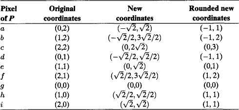
A naive approach to applying the geometric transformation of Equation 14.1 to a picture P would be as follows. For each pixel of P (e.g., at location (x,y)), compute its new coordinates (x′,y′) using Equation 14.1; round these coordinates to the nearest integers [x′], [y′]; and construct a new picture P′ in which the pixel at location ([x′], [y′]) has value P(x,y). Unfortunately, this naive approach would lead to unacceptable results; it would assign no values to some pixels of P′ and more than one value to other pixels. To see this, consider a simple example in which we apply a 45° counterclockwise rotation to the 3 × 3 picture P that has pixel values that are shown in Figure 14.2. This rotation takes (x,y) into the point that has the following coordinates:

Let the center of rotation and the origin be at the pixel that has value g; then the new coordinates of the nine pixels and their rounded values are as shown in Table 14.1. Thus the pixels at locations (−1,1) and (1,1) each get two values (a and d, h and i), and the pixel at location (0,2) gets no value, even though it is surrounded by pixels that do get values. Schematically, the new picture looks like Figure 14.3.

Evidently, the rounded 45° rotation is not a one-to-one correspondence of the grid with itself. For example, when we apply it to a DSS consisting of five diagonally consecutive pixels, we obtain five pixels that lie on a horizontal (or vertical) line, where they occupy an interval of length ![]() ; thus the five original pixels rotate into five out of seven horizontally consecutive pixels. Two of these seven pixels will have no values assigned to them, so the rotated line segment will have gaps. Conversely, when we rotate a horizontal DSS consisting of seven horizontally consecutive pixels, the rotated pixels occupy an interval of length
; thus the five original pixels rotate into five out of seven horizontally consecutive pixels. Two of these seven pixels will have no values assigned to them, so the rotated line segment will have gaps. Conversely, when we rotate a horizontal DSS consisting of seven horizontally consecutive pixels, the rotated pixels occupy an interval of length ![]() on a diagonal; thus the values of the seven original pixels must be assigned to five pixels, so two of these pixels will have more than one value assigned to them.
on a diagonal; thus the values of the seven original pixels must be assigned to five pixels, so two of these pixels will have more than one value assigned to them.
We can avoid these difficulties by using the inverse of the transformation in Equation 14.1 to map each pixel in the new picture (e.g., with coordinates (x′,y′)), into a (real) point (x, y) in the plane that contains the original picture P. (We are assuming that the transformation in Equation 14.1 is invertible.) Let the inverse of the transformation in Equation 14.1 be as follows:
It specifies the old coordinates of a point as functions of the point’s new coordinates. Equation 14.2 maps (x′,y′) into a point (x″,y″) in the plane of the old picture P.
We assign a value to the pixel of the new picture at location (x′,y′) by interpolating between the values of the pixels of P that lie near (x″,y″). Alternative methods of performing this interpolation will be discussed shortly; for the moment, we will use nearest-neighbor (sometimes called zero-order) interpolation, in which (x′,y′) is given the value of the pixel of P that lies closest to (x″,y″).
When we use the inverse transformation and nearest-neighbor interpolation, our rotation example works as follows. The inverse transformation is a clockwise 45 rotation that takes (x′,y′) into the point that has the following coordinates:
When we apply this transformation, the nearest-neighbor values for the pixels of P′ are as shown in Table 14.2. Note that the same value is assigned to more than one pixel (both (0,1) and (0,2) get e), and some of the values (a and i) are not assigned to any pixel; however, every pixel in P′ gets a unique value, as shown in Figure 14.4.

As we see from Figure 14.4, the rotated picture is no longer an upright square; it is approximately a 45° rotated square. In general, if we want to display a geometrically transformed picture on a finite square grid, we may have to leave parts of that grid (such as its corners) blank, or we may have to discard the values of parts of the original picture. If the transformation is not continuous, the transformed picture may not even be connected!
We now consider alternative methods of performing the interpolation. The simplest such method is bilinear interpolation, which is defined as follows. Let the integer parts ![]() x″
x″![]() ,
, ![]() y″
y″![]() of x″ and y″ be i and j so that (x″,y″) is surrounded by the four grid points having coordinates that are shown in Figure 14.5. Let the fractional parts of x″ and y″ be α = x″ –
of x″ and y″ be i and j so that (x″,y″) is surrounded by the four grid points having coordinates that are shown in Figure 14.5. Let the fractional parts of x″ and y″ be α = x″ –![]() x″
x″![]() and β = y″ –
and β = y″ –![]() y″
y″![]() ; thus 0 ≤ α, β < 1. Then the value that we assign to the pixel at location (x′,y′) is as follows:
; thus 0 ≤ α, β < 1. Then the value that we assign to the pixel at location (x′,y′) is as follows:

Note that, if x″ is an integer (i.e.,α = 0), (x″, y″) is on the line segment between pixels (i, j) and (i, j + 1), and a value is assigned to (x′,y′) by linear interpolation between their values: (1 –β)P + βP(i,j + 1). Similarly, if y″ is an integer, we have β = 0; here (x″,y″) is collinear with (i,j) and (i + 1,j), and (x′,y′) gets value (1 –α)P(i,j) + αP(i + 1,j). Finally, if x″ and y″ are both integers, we have α = β = 0 and (x″, y″) = (i,j) so that (x′,y′) gets value P(i,j) as would be expected.
To illustrate this method, we again consider our rotation example. Here the values to be assigned to the pixels of the new picture are determined as shown in Table 14.3. All nine of the original values now contribute to the values of the new pixels, although two of them (a and i) do not make the largest contribution to the value of any pixel, and e makes the largest contribution to the values of two different pixels. No values get entirely discarded, but only one of the old values (g) is preserved exactly, and the other values are blurred or attenuated. Note that the inverse transforms of (0,3), (1,2), and (−1,2) lie slightly outside of the old 3 × 3 grid, so some of the pixels that surround their preimages (x″, y″) are “blank” (indicated in Table 14.3 by hyphens). When computing the values for the pixels at (0,3), (1,2), and (−1,2), we have treated the blanks as having value 0.

Higher-order interpolation schemes can also be used; these generally yield better-appearing results. For example, we can use bicubic spline interpolation,in which the pixel values are approximated by a linear combination of products of cubic polynomials ΣΣCijgi(x)gj(y). The coefficients of these polynomials can be chosen so that the approximation is an exact fit to the values at the pixel locations. The details will not be given here.
The preferred interpolation scheme depends on the nature of the transformation and on the type of picture that is being transformed. For example, if P is a binary picture that has only values 0 and 1 (representing black and white), we might prefer to use nearest-neighbor interpolation, because the higher-order interpolation methods introduce intermediate values, which may be of no interest. As another example, suppose we are magnifying a picture using a transformation of the following form, where k ![]() 1:
1:
Nearest-neighbor interpolation would assign the same values to large blocks of pixels in the magnified picture (e.g., magnification of our 3 × 3 picture using k = 3 would give the 9 × 9 array shown in Figure 14.6); this blocky appearance would usually be objectionable. If we use bilinear interpolation, the pixel values of the magnified picture would be as shown (in part) in Figure 14.7; thus the picture would have a smoother appearance. A real picture that has been magnified by a factor of 10 using nearest-neighbor, bilinear, and bicubic interpolation is shown in Figure 14.8; note that very little improvement is obtained by using bicubic interpolation.


FIGURE 14.8 10 × magnification of part of a picture using (left) nearest-neighbor interpolation, (middle) bilinear interpolation, (right) bicubic interpolation.
Conversely, if we demagnify a picture (i.e., k ![]() 1) using low-order interpolation, the pixel values in the demagnified picture depend only on a few of the old pixel values in the vicinities of the preimages of the new pixels; many of the old pixel values will have no influence on the demagnified picture. If we do not want to discard these old values completely, we should use an interpolation scheme in which the pixels in a large neighborhood of the preimage of a new pixel contribute to the value of that pixel.
1) using low-order interpolation, the pixel values in the demagnified picture depend only on a few of the old pixel values in the vicinities of the preimages of the new pixels; many of the old pixel values will have no influence on the demagnified picture. If we do not want to discard these old values completely, we should use an interpolation scheme in which the pixels in a large neighborhood of the preimage of a new pixel contribute to the value of that pixel.
Interpolation may be necessary even if the geometric transformation is a translation x′ = x +α, y′ = y +β. If the translation is by an integer amount, no interpolation is needed; otherwise, bilinear interpolation is appropriate. Interpolation is also unnecessary when a picture is rotated around a grid point by a multiple of 90° or reflected in a grid line; linear interpolation is appropriate when a picture is reflected in a (non-grid) horizontal or vertical line.
When we use nearest-neighbor interpolation, a geometric transformation takes binary pictures into binary pictures but may not preserve geometric properties of the pictures. For example, we saw in Figure 14.4 that the result of rotating the nine-pixel picture by 45° had only eight pixels; thus the rotation did not preserve area. Similarly, 45° rotation of a five-pixel diagonal DSS yields a seven-pixel horizontal or vertical DSS (and vice versa). Moreover, the horizontal or vertical segment is 4-connected, but the diagonal segment is only 8-connected; thus the rotation does not even preserve topology. Evidently, translation does preserve geometric properties, and magnification or demagnification evidently does not preserve area. Magnification preserves topology (a magnified connected or disconnected set is evidently still connected or disconnected), but demagnification apparently cannot preserve disconnectedness, because distant pixels may become neighbors.
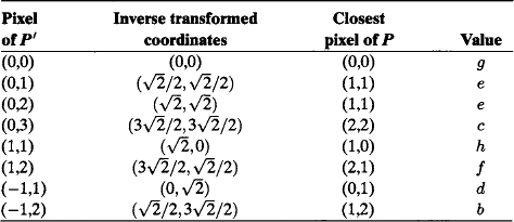
A general geometric transformation of the plane can be approximated by, for example, linear transformations that are defined on small pieces of the plane. For example, we can divide the plane into small squares and use a linear transformation on each square; this maps the square into a quadrilateral. If the transformations of adjacent squares agree at the common vertices of the squares, these quadrilaterals will “fit together” to tessellate the plane. An historic example of a piecewise linear geometric transformation that converts a distorted grid of lines into an undistorted grid is shown in Figure 14.9.
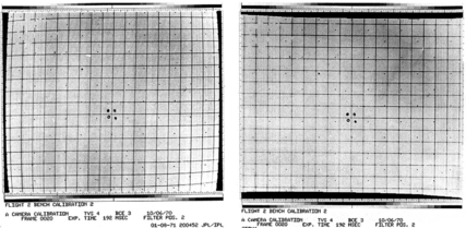
FIGURE 14.9 Conversion of a distorted grid of lines (left) into an undistorted grid (right) using a piecewise linear geometric transformation. (from [784])
14.6 Magnification and Demagnification
As we saw in Section 14.5, magnification of a picture P by an integer factor k ≠ 1 replaces each pixel p of P with a k × k block of pixels. We can think of the new pixels (in the grid cell model) as having the same size as the original pixels; this implies that the height and width of the new picture are k times those of the original picture and that the area of the new picture is k2 times that of the original picture. Alternatively, we can think of the new picture as being obtained by subdividing each pixel of the original picture into a k × k block of “mini-pixels,” each of which has height and width 1/k and area 1/k2 (if the original pixels were of unit size). k-fold magnification using this alternative approach is equivalent to redigitizing P on a grid of resolution k (see Chapter 2) and using nearest-neighbor interpolation.
In the grid cell model, a (nonextremal) 0-cell is contained in four 1-cells and four 2-cells; a 1-cell contains two 0-cells and (if it is nonextremal) is contained in two 2-cells; and a 2-cell contains four 0-cells and four 1-cells. When we perform k-fold magnification, a magnified 1-cell contains (k + 1) 0-cells and k unit 1-cells; a magnified 2-cell contains (k + 1)2 0-cells, 2k(k + 1) unit 1-cells, and k2 unit 2-cells.
If we use outer Jordan digitization (in the grid cell model), an α-arcρ in P is a sequence of cells p0,p1,…,pn such that pi is α-adjacent to pi−1(1 ≤ i ≤ n). k-fold magnification converts ρ into a sequence of k × k blocks of cells p0, p1,…, pn such that pi is α-adjacent to pi−1(1 ≤ i ≤ n); we can think of the magnifiedρ as a “thick” arc. If we use grid-intersection digitization,ρ is a sequence of grid points. The vector vi = pi−1pi is either an isothetic unit vector or a diagonal vector of length ![]() . Let vi make angle 45i° with the positive x-axis; then vi can be represented by the chain code i ∈{0,…,7}, and ρ can be represented by a chain code sequence i0,i1,…in. It is not hard to see that the k-fold magnification ofρ has the chain code
. Let vi make angle 45i° with the positive x-axis; then vi can be represented by the chain code i ∈{0,…,7}, and ρ can be represented by a chain code sequence i0,i1,…in. It is not hard to see that the k-fold magnification ofρ has the chain code ![]() , where ik denotes k-fold repetition of i [342].
, where ik denotes k-fold repetition of i [342].
Demagnifying a picture cannot preserve all of its pixel values, but it provides a “summary” of the picture that may be useful for many purposes. Even when a picture is substantially demagnified, its gross structure usually remains quite recognizable; the demagnified picture is a “miniature” (sometimes called a “thumbnail”) of the original. Figure 14.10 shows three pictures and the results of demagnifying them by a factor of 8. The demagnified pictures are also shown remagnified (by factors of slightly less than 8, using nearest-neighbor interpolation) to illustrate the information that is still available after eightfold demagnification.
Different degrees of demagnification may be useful for different purposes, depending on what information about the original picture needs to be preserved. It may therefore be desirable to use a set of demagnifications (e.g., by powers of 2) so that any desired demagnification is approximated by one of them. Figure 14.11 shows demagnifications of a 512 × 512 picture by successive powers of 2 (from 2 to 512).
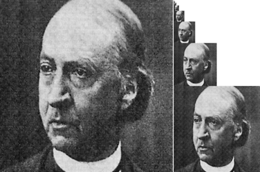
FIGURE 14.11 Demagnification of a 512 × 512 picture (of J.B. Listing) by factors of 2, 4, 8, 16, 32, 64, 128, 256, and 512.
If the size of the original picture (in pixels) is 2n × 2n, its demagnifications by powers of 2 have sizes 2n−1 × 2n−1, 2n−2 × 2n−2, and so on. The total number of pixels in all of these demagnified pictures is less than the following (i.e., less than ![]() more than in the original picture):
more than in the original picture):
This succession of demagnified versions of a picture can be thought of as a “pyramid” of pictures; note that this pyramid “tapers” exponentially rather than linearly.
From a picture of size 2n × 2n, we can construct an n + 1-level pyramid in which level k is a picture of size 2k × 2k (0 ≤ k ≤ n). In this pyramid, the value of a pixel p on any level k <n is the average of the values of a 2 × 2 block of pixels on level k + 1. The value of the single pixel on level 0 is the average of the values of all of the pixels of the original picture, the values of the four pixels on level 1 are the averages of the values of the pixels in the four quadrants of the original picture, and so on.
We can construct a rooted tree of degree 4 in which the pixel on level 0 is the root and each pixel p on any level k < n is linked to its four “children” (a 2 × 2 block of pixels) on level k + 1. The leaves of this tree are the pixels of the full-size picture at the base of the pyramid. Using this pyramid structure, we can explore the picture at any given scale by moving between adjacent pixels on a given level, and we can explore it in (discrete) scale-space by moving between parents and children on consecutive levels. The structure of a three-level pyramid is shown in Figure 14.12.

Demagnification of a picture is not a translation-invariant operation; the results depend on the positions of the blocks of pixels that are represented by single pixels in the demagnified picture. For example, consider the one-dimensional binary picture with the following pixel values:
Suppose we demagnify this picture by a factor of 2 so that the pixels at locations x and x + 1(x = …, −2, 0, 2, 4,…) are represented by a single pixel. If the coordinate of the rightmost 1 is odd, the demagnification yields …,1,1,0,0,…; however, if this coordinate is even, the demagnification yields …1,1,![]() ,0,0,…. As an extreme example, consider the following picture:
,0,0,…. As an extreme example, consider the following picture:
If the righthand 1s have odd coordinates, demagnification by a factor of 2 yields …,1,0,1,0,1,…; if they have even coordinates, it yields …,![]() ,
,![]() ,
,![]() ,
,![]() ,
,![]() ,…
,…
The position-dependence of the effects of demagnification can be reduced by smoothing the picture before demagnifying it. Smoothing is accomplished by replacing the value of each pixel with a weighted average of the values of the pixel and some of its neighbors. If the pixel at coordinate x in a one-dimensional picture has value P(x) the weighted averaging gives it the following new value:
(This is a weighted average of the values of an odd number of pixels; averaging neighborhoods of even sizes can also be used.) The weights should satisfy the following conditions:
(1) ![]() : This ensures that the weighting process does not result in an increase or decrease in the average value of the pixels. To further ensure that each pixel of P contributes the same total weight to each pixel of
: This ensures that the weighting process does not result in an increase or decrease in the average value of the pixels. To further ensure that each pixel of P contributes the same total weight to each pixel of ![]() , we require that the sums of the ws in even-numbered and odd-numbered positions both be
, we require that the sums of the ws in even-numbered and odd-numbered positions both be ![]() .
.
(2) w–k = wk for all 1 ≤ k ≤ m: The weights are symmetric.
(3) ![]() for all 0 ≤ k < k′ ≤ m: The center weight is the highest, and the weights decrease as they get farther from the center.
for all 0 ≤ k < k′ ≤ m: The center weight is the highest, and the weights decrease as they get farther from the center.
For m = 2, there are five weights; because they are symmetric, we can denote them by γ,β,α,β,γ where γ ≤β ≤α. Condition (1) implies that α + 2β + 2γ = 1 and ![]() , so
, so ![]() . Condition (3) requires that
. Condition (3) requires that ![]() ,so
,so ![]() . If we require the weights to be nonnegative, we must have
. If we require the weights to be nonnegative, we must have ![]() , but we are still free to choose α in the range
, but we are still free to choose α in the range ![]() . In our extreme example,
. In our extreme example,
if we smooth using weights for which ![]() and
and ![]() , the value of the smoothed picture at the 1s is
, the value of the smoothed picture at the 1s is ![]() , and its value at the 0s is
, and its value at the 0s is ![]() ; thus the smoothed picture is constant, so its demagnification is no longer position-dependent. In 2D, it is usual to require that the weights wjk be separable (i.e., wjk = wjwk).
; thus the smoothed picture is constant, so its demagnification is no longer position-dependent. In 2D, it is usual to require that the weights wjk be separable (i.e., wjk = wjwk).
14.7 Digital Tomography
Section 1.2.11 defined digital tomography in very general terms. To be more specific, assume (see Section 14.2) a digital geometry on Zn (n ≥ 2) and a set T of translations on Zn (e.g., translations in isothetic directions).
Let D = {γ(1)…,γ(m)} (m ≥ 1) be a set of pairwise nonparallel (see Proposition 14.1) lines in Zn. Each line is uniquely determined by a grid point p ∈ Zn and a generator Φ ∈ T.
Let Γi be the set of lines in Zn that are parallel to γ(i) (1 ≤ i ≤ m). The equivalence class Γi is a direction in the set of all lines. Zn and T satisfy axiom G8 (i.e., we can enumerate the lines in ![]() , where
, where ![]() for some k ∈ Z).
for some k ∈ Z).
Figure 14.13 shows an example in which n = 2 and T is the set of translations along the x- or y-axis. For a finite set S, we have nonzero projections Pi(j) only in finite intervals of j-values. Let I1 × … × Im be the smallest cuboidal subset of Zn that covers all of the nonzero projections. The reconstruction problem in digital tomography is as follows: given a set P = (P1,…,Pm) of projections in specified directions, find a finite set S ⊂ Zn (n> 2) that has the given projections.

FIGURE 14.13 Left: two projections of a column-convex polyomino. Middle and right: corresponding system of linear equations.
The reconstruction problem for the set shown in Figure 14.13 has a unique solution; the corresponding system of linear equations (which identifies each pixel in I1 × … × Im with a variable xk ∈ {0,1}), where k = 1,…, 16, has only one solution.
A possible method of solving the reconstruction problem of digital tomography is to apply algorithms of computed tomography (CT) [215] (e.g., algorithms based on Fourier transforms [implementing the inverse Radon transform] or iterative reconstruction algorithms). However, these algorithms calculate real values at pixel positions. The algebraic reconstruction technique (ART) of [372] can be modified to yield a binary solution [423, 170]. Linear programming provides other alternatives (simplex method, interior point methods); see [381].
We conclude this section by discussing the reconstruction of a binary picture (matrix) from two projections, as illustrated in Figure 14.13. The input P = {R, S} is a pair of projections in the row and column directions. In Figure 14.13, we have R = (3,3,1,1) and S = (2,3,2,1). Two vectors R =(r1,…,rm) and S =(s1,…,sn) are compatible iff they contain only nonnegative integers ri ≤ n (i = 1,…,m) and sj ≤ m, (j = 1,…,n) and the sum of the ris equals the sum of the sjs.
The solvability of a reconstruction problem defined by a pair of compatible vectors {R, S} is characterized by the following theorem, independently discovered by H.J. Ryser [934] and D. Gale [350] in 1957. We permute the vector ![]() such that
such that ![]() . We define an m × n matrix
. We define an m × n matrix ![]() in which row i consists of ri 1s followed by n – ri 0s. Let
in which row i consists of ri 1s followed by n – ri 0s. Let ![]() be the projection vector of
be the projection vector of ![]() in the column direction.
in the column direction.
Theorem 14.4
The reconstruction problem for R =(r1,…, rm) and S = (s1,…, sn) has at least one solution (a binary picture of size n × m) iff the following is true:
The case k = 1 is already covered by the compatibility of the vectors R and S. In our example, we have S′ = (3,2,2,1) and ![]() , where 5 ≥ 4 for k = 2, 3 ≥ 2 for k = 3, and 1 ≥ 0 for k = 4.
, where 5 ≥ 4 for k = 2, 3 ≥ 2 for k = 3, and 1 ≥ 0 for k = 4.
A switching component of a binary picture is a 2 × 2 block of pixels of the following form:
If a picture has a switching component, it is evidently not uniquely reconstructible from its row and column projections. In [934], Ryser proved the following:
Note that additional knowledge about the given binary picture (e.g., that it contains only one row-convex, column-convex, or convex polyomino) may allow a unique reconstruction that would not otherwise be possible.
14.8 Exercises
1. The set of all geometric transformations of the plane is closed under composition of functions; if f :(x′ = h1(x,y), y′ = h2(x,y)) and g :(x′ = k1(x,y), y′ = k2(x,y)) are geometric transformations, then g o f (x″ = k1(h1(x,y), h2(x,y)), y″ = k2(h1 (x,y), h2(x,y))) is also a geometric transformation. Composition of functions is associative (i.e., for all f, g, h, we have (f o g) o h = f o (g o h)). The identity transformation i :(x′ = x, y′ = y) is an identity element for the composition of geometric transformations (i.e., for all f, we have i o f = f o i = f). g is called an inverse of f if g o f = f o g = i. A set G of geometric transformations of the plane is called a group if G contains i and any f ∈ G has an inverse in G. Prove that the following sets of transformations are groups:
(2) {i,rx}, {i,ry}, and {i,ro} where rx,ry, and ro are the reflections in the x-axis, the y-axis, and the origin
(3) {i,rx,ry,r1,r2} where r1 and r2 are the reflections in the two diagonals
(4) {i,rπ} where rπ is the rotation around the origin by 180°
(5) {i,rπ/2,r–π/2,rπ} where rπ/2 and r–π/2 are the rotations around the origin by ±90°
(6) {i,rπ/2,r–π/2,rπ,rx,ry,r1,r2}
2. Prove that a rotation by angle θ around the origin (0,0) is defined by the following pair of equations:
3. The reflections in the x-axis, the y-axis, and the origin are defined (respectively) by the following pairs of equations:
Prove that these reflections are not the same as rotations through any angle around the origin.
4. Write the equations for reflection in a line L through the origin that makes angle θ with the x-axis using the fact that this reflection can be accomplished by rotating L (through angle –θ) until it coincides with the x-axis, then reflecting in the x-axis, and then rotating back through angle θ.
5. An affine transformation is defined by the following equations, where a1b2 ≠ a2b1:
Prove that translations, rotations, reflections, and scale changes (magnifications or demagnifications) are all affine transformations.
6. Characterize affine transformations that consist of a translation followed by a rotation (or vice versa). Such a transformation is called a rigid motion. Two pictures that differ by a rigid motion are called congruent. (Note that most rigid motions do not take pixels into pixels. Thus mapping a picture into a picture by a rigid motion requires interpolation; the pixel values in two pictures that differ by a rigid motion may not be the same.) Two pictures that differ by a rigid motion followed by a scale change (or vice versa) are called similar.
7. A shear is a transformation defined by the equations x′ = x + ay, y′ = y or x′ = x, y′ = y + ax; thus a shear takes pixels into pixels iff a is an integer. Prove that a shear cannot be d-continuous unless it is the identity (a = 0).
8. Let R be a bounded region of the plane, and let f be a d-continuous function from Z2 into Z2 that takes pixels in R into pixels in R. Prove that there must exist a pixel p in R such that d8(p,f (p)) ≤ 1.
9. Show that the converse of Proposition 14.4 is not always true for de.
10. Generalize the results of Section 14.4 to 3D.
11. The group of one-to-one geometric transformations of pictures P defined on Gn,n (n ≥ 3) consists of eight transformations: the identity id; the vertical, horizontal and diagonal reflections ver, hor, and dia; the 90°, 180°, and 270° (clockwise) rotations rot, rot2, and rot3; and a transformation mir defined by mir(P) = rot(hor(P)) that satisfies mir(P) = ver(rot(P)) = dia(ver(hor(P))). Construct a table of all compositions op1(op2(P)) of pairs of these transformations, and show that this table proves that these transformations form a group.
12. In the 3D grid cell model, a nonextremal 0-cell is contained in six 1-cells, 12 2-cells, and eight 3-cells; a 1-cell contains two 0-cells and (if it is nonextremal) is contained in four 2-cells and four 3-cells; a 2-cell contains four 0-cells and four 1-cells and is contained in two 3-cells; and a 3-cell contains eight 0-cells, 12 1-cells, and six 2-cells. How many 0-cells, unit 1-cells, unit 2-cells, and unit 3-cells are contained in a k-fold magnified 3-cell?
14.9 Commented Bibliography
The introductory remarks about the history of geometry follow [544]. Geometry is one of the best axiomatized disciplines in mathematics [334, 384]. For definitions of discrete geometry, see [96, 319, 394]. The conferences on “Discrete Geometry for Computer Imagery,” of which [111] was the first held outside France, actually focus on digital geometry.
The habilitation [449] of A. Hübler, which unfortunately has remained unpublished except for some small notes such as [450], contains valuable contributions to the definition and analysis of the translation group T of digital geometry and the axiomatic foundations of digital geometry on the regular orthogonal grid in Rn. See also the essay [1009] about the axiomatic foundations of convexity and linearity. Hübler’s axiomatic theory was recently studied in [228].
Symmetry groups in geometry are discussed, for example, in [221, 704, 1008, 1122]. Digital symmetry, as discussed in Section 14.3, is further detailed in [486]; see also [863]. For accumulator space-based symmetry analysis of “noisy” planar polygons, see [463]. [267] discusses symmetry analysis in pyramidal picture representations.
For Exercise 11, see [533], which also studied the cardinalities of families of geometric transformations defined on Gn,n(n ≥ 2), including magnifications, demagnifications, shifts, and cyclic shifts, as well as the cardinalities of (see the definition in Section 17.7) families of local operations of order k ≥ 1. For geometric constructions in the digital plane, see [1090].
d-continuous functions on Z2 were introduced in [903]. For “continuous” functions on nonbinary pictures, see [766]. For digital versions of homeomorphism, retraction, and homotopy, see [114]. A “calculus” for d-continuous functions is discussed in [767].
Methods of applying geometric transformations to pictures were discussed in [477] and were used for the geometric correction of pictures in [784]. For another method of digital rotation, see [21].
For magnification by an integer factor, see [1107]. [524] proves that Hough transforms based on real spaces are superior (with respect to the size of the accumulator array) to “digital Hough transforms.”
The pyramid data structure was introduced in [1045]. For a collection of papers about multiresolution picture representation and processing, see [899]. For methods of smoothing a picture prior to reducing its resolution, see [154]. Uses of pyramids in picture analysis and computer vision are discussed in [479]. A pyramid is a discrete version of a scale-space in which scale varies continuously; see [652].
In the pyramids described in Section 14.6, the value of each pixel on level k is the average of a 2 × 2 block of pixels on level k + 1. More generally, we can construct pyramids in which each pixel value on level k is a weighted average of a block of pixel values on level k + 1, where the blocks can overlap and can be of any desired size (or shape). Still more generally, for any graph G, we can construct a pyramid of graphs G0,G1,…,Gn in which Gn = G, each node of Gk (k < n) is linked to the nodes of a subgraph of Gk + 1, and every node of Gk + 1 belongs to one of these subgraphs. [551] discusses repeated derivation of region-adjacency graphs, layer by layer, starting with a general adjacency graph. If values are associated with the nodes of G, we can give each node p of each Gk a value that is a function of the values of the nodes of the subgraph of Gk + 1 to which p is linked. We can also identify each node of Gk with a “representative” node of Gk + 1 (i.e., we can regard Gk as being obtained by the “reduction” of Gk + 1). For a recent review of such general methods of constructing pyramids and the uses of such pyramids in picture analysis, see [478]. Pyramidal approaches are also closely related to multiscale representations of shapes. [70] discusses representations of borders of regions at different scales in terms of DSSs, circular arcs, corners, and points that delimit the arcs.
Section 14.7 reviews parts of Chapter 1 (by A. Kuba and G.T. Herman) of [431], which is a collection of papers about discrete (particularly, digital) tomography; see also [380]. Theorem 14.4 is from [350, 934]. The proof of this theorem involves an algorithm that constructs a solution in O (n (m + log n)) time. For the reconstruction of pictures from multiple projections (a combinatorial subject), see [58, 60, 141, 142, 261, 353, 354, 355]. The reconstruction of isothetic polygons from labeled (convex or concave) vertices is discussed in [629].
1]A set of axioms is consistent iff it is impossible to deduce a contradiction from it; it is nonredundant iff none of the axioms can be deduced from the others; and it is complete iff it can be used to prove or disprove every proposition.
2]Parallel publications in 1891 by E.S. Fedorov [317], a director of mines in the Ural region, and A. Schönflies [966], a professor at Göttingen University, classified all 230 symmetry groups of crystal in 3D space. Their results were in close agreement, and Schönflies granted Fedorov priority for the discovery [153].
3]See the picture gallery “Symmetry” at http://www.mcescher.com/.