
3D Straightness and Planarity
This chapter discusses digital straightness in 3D space, thereby generalizing the DSS- and MLP-based concepts, models, and algorithms that were studied in Chapters 9 and 10 It also discusses digital planarity in the 3D grid adjacency and incidence models, including relationships with other disciplines. Algorithms for recognizing digital planar segments are briefly reviewed, and one algorithm for partitioning a digital surface into such segments is discussed in detail.
11.1 3D Straightness
A digital straight line (DSL) in Z3 can be defined by 3D grid-plane intersection digitization, arithmetic geometry, or outer 3D Jordan digitization of a straight line γ ⊂ R3. It can be treated in 3D grid adjacency models or in the 3D grid incidence model, which is based on 0-, 1-, 2-, and 3-cells (see Section 11.1.4).
11.1.1 Grid-plane intersection digitization
Using the approach in Section 2.3.5, the 3D grid-plane intersection digitization of γ in ![]() is
is ![]() where the following is true:
where the following is true:
γ can intersect a grid plane in such a way that up to four grid points are closest to the intersection point. As is the case in 2D grid-intersection digitization, we exclude such cases by selecting one of these grid points using some decision rule. The resulting 3D DSL is the doubly infinite sequence …,q−1,q0,q1,… of center points (grid points in Z3) of the 3-cells in ![]() ).
).
A (26-) DSL segment (3D DSS or 26-DSS) is a finite subsequence of a 3D DSL. Evidently, a 3D DSS is a simple 26-arc. Arational 3D DSL is the digitization of a rational straight line γ = {(βx +αxt, βy +αyt, βz +αzt): t ∈ R}; here β = (βx,βy,βz) ∈ R3 can be arbitrary, but the slopes αx,αy, and αz must be rational.
The conditions for 2D straightness discussed in Chapter 9 can be extended to 3D. For example, S ⊆ Z3 has the chord property, iff for any p,q ∈ S, every point on the straight line segment pq ⊂ R3 is at L∞ -distance < 1 from some point of S. (We recall that the Minkowski metric L∞ coincides with d26 on Z3.) It can be shown [511] that a simple 26-arc is a 3D DSS iff it has the chord property. In [511], the following theorem is also proved:
Either of these projections may be a single grid point; the third projection may not even be a simple 8-arc. Figure 11.1 illustrates projections of 26-DSSs.

FIGURE 11.1 Segmentations of a 26-arc (left) and a 26-curve (right) into maximum-length 26-DSSs (ending at black voxels), together with their projections into the (x = 0)-, (y = 0)-, and (z = 0)-planes [203].
Theorem 11.1 provides a straightforward method of recognizing 26-DSSs and, therefore, of segmenting a 26-arc into a sequence of maximum-length 26-DSSs. We project the given 26-arc onto the three planes and apply 8-DSS recognition to the projections; we continue as long as 8-DSS recognition is successful for at least two of the projections.
11.1.2 Arithmetic geometry
3D DSSs are defined in arithmetic geometry by linear Diophantine inequalities; see Section 9.2. A 3D digital line is characterized by relatively prime integers a, b, and c (where 0 ≤ c ≤ b ≤ a) that correspond to the coordinates x, y, and z in that order. For other orders of a, b, and c, we can permute the coordinates.
Definition 11.1
G ⊂ Z3 is a 3D arithmetic line defined by integers a, b, c, μ1,μ2,ω1, and ω2 iff the following is true:
The parameters μ1 and μ2 are called the lower bounds of G, and the parameters ω1 and ω2 define its arithmetic thickness.
LetG be a 3D arithmetic line defined bya, b, c,μ1,μ2,ω1,ω2 ∈ Z where 0 ≤c < b <a. Then the following are true:

G is called a 3D naive line iff ω1 = ω2 = max{|a|, |b|, |c|} = a. When c = 0, G is a (2D) naive line, as in Chapter 9 If c> 0, in accordance with Equation 11.4, G is 26-connected. c ≤ b ≤ a corresponds to the following parameterization of G, using parameter x only:
Evidently, a 3D naive line is an unbounded simple 26-arc. It is provided in [203] that the following is true:
This theorem and Theorem 11.1 imply the following:
11.1.3 A linear online 3D DSS segmentation algorithm
Corollary 11.1 justifies the following 3D DSS segmentation algorithm, which uses the (C2.1a) approach that was defined in Chapter 9 (Theorem 9.4) and that was originally published in [256].
We consider a projection of the given 26-curve into one of the (x = 0)-, (y = 0)-, or (z = 0)-planes. Without loss of generality, assume an 8-curve in the (z = 0)-plane; this allows us to suppress the z-coordinate. The grid points (x, y) on a DSS must satisfy the following condition,
where a and b are relatively prime integers and μ is an integer. We describe the calculation of a, b, and μ.
Algorithm DR1995
The initial grid point q1 of a new 8-DSS can be chosen as the origin. It is sufficient to implement the algorithm for the first octant (i.e., slope in [0,1)); other cases can be mapped into this case by reflection. At q1 = (0,0), we start with condition D1 : 0 ≤ –y < 1 (i.e., a = 0, b = 1, and μ = 0). We assume that the given sequence of grid points involves moves in at most three directions: (1,0), (1,1),or (1,-1); thus we proceed in the x-direction in the first octant.
The points qi = (ai,bi), where 1 ≤ i ≤ n, form an 8-DSS or a segment of a naive line iff (see Theorem 9.4) there are relatively prime integers a and b with a <b (recall that we are assuming the first octant) and an integer v such that all n points are between or on a lower supporting line ax – by = μ and an upper supporting line ax – by = μ + max {|a|, |b|} −1 = μ + b − 1 (note again that we are in the first octant). For a new point qn + 1 ∈ A8(qn), where xn + 1 > xn, we have three cases: qn + 1 is between or on these two lines (i.e., no update is needed) or it is (“just”) above the upper or (“just”) below the lower supporting line.
[253, 256] give simple decision and updating criteria for these cases. Let u1,u2 and l1, l2 be the points on the upper and lower supporting line, respectively, where index 1 denotes the point qi (1 ≤ i ≤ n) with the smallest x-coordinate and index 2 denotes the point with the largest x-coordinate (compare points StartN, EndN and
StartP, EndP in Figure 9.7). Let r = axn + 1 – byn + 1 be the remainder of point qn + 1 with respect to the slope a/b of the given naive line segment {q1,…,qn}⊂ Da,b,μ,–b.
The theorem translates into an 8-DSS algorithm, which is shown in Algorithm 11.1.
Figure 11.2 shows a sequence qi = pi – p1 where, in the first octant, p1 = (1,2) and i = 1,…, 11. q1 and q2 satisfy condition D2 : 0 ≤ x – y < 1 with μ = 0; the upper supporting lines are both y = x. q1, q2, and q3 satisfy condition D3 : −1 ≤ x − 2y < 1; here, the lower supporting line is 2y = x, and μ = −1 is defined by q2. At q6 = (5,2), we have condition D6 : −4 ≤ 2x − 5y < 1;μ = −4, a = 2, and b = 5, and the upper supporting line is defined by q4. At q10, we still have a naive line segment q1,…,q10 with l1 = q1, l2 = q6, u1 = q4, and u2 = q9. The remainder r at q11 is −5 (i.e., we have the second case in Theorem 11.3). The new slope is defined by vector u1q11 = (7,3), and {q1,…,q11} is a segment of the naive line D11 : −5 ≤ 3x – 7y < 2. We now have l1 = l2 = q6, u1 = q4 and u2 =q11.
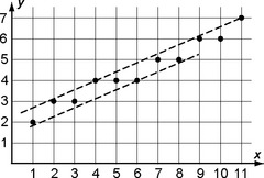
Figure 11.3 shows a circle and an ellipse in general 3D positions (in the grid cell model) and their DSS segmentations.

FIGURE 11.3 Examples of DSS segmentations; the windows (gray) are magnified to show details. The curves do not lie in planes parallel to the (x = 0)-, (y = 0)-, or (z = 0)-plane. Left: a circle. Right: an ellipse [203].
Suppose we successfully apply a DSS recognition algorithm in two of the coordinate planes, for example, by obtaining supporting lines in the (y = 0)-plane with normal ny = (y1,y2) and in the (z = 0)-plane with normal nz = (z1,z2); then these two 8-DSSs are projections of a 26-DSS that has normal n = (y2z2,y2z1,y1z2). Note that, if (y1,y2) and (z1,z2) are 2D grid points with relatively prime integer coordinates, the coordinates of n need not be relatively prime.
Figure 11.4 illustrates the linear run time of the 3D DSS segmentation algorithm and shows two successful 2D DSS segmentations for each segment in 3D space.
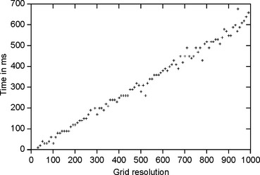
FIGURE 11.4 Run time (in ms) of the 3D DSS segmentation procedure on a Sun Ultra SparcStation [203] for a digitized circle in 3D space; see the left side of Figure 11.3.
11.1.4 MLPs of simple 2-curves
In this section, we consider DSLs in the 3D incidence grid. The outer 3D Jordan digitization of a straight line γ ⊂ R3 is a finite set of 3-cells. We also use grid vertices, edges, and faces in the following discussion. We assume that γ is not incident with any grid vertex; it follows that the DSL is a 2-arc in the 3D grid cell model.
A 2-curve in C3 can be represented as an alternating sequence ρ = (f0,c0,f1,c1, …,fn,cn) of faces fi and cubes ci (0 ≤ i ≤ n) such that fi and fi + 1 are sides of ci and fn + 1 = f0. A 2-arc ξ is a 2-connected subsequence of 3-cells starting at a face fi and ending at a face fj ≠ fi. Evidently,ξ is a DSL (with respect to outer 3D Jordan digitization) iff there is a straight line segment in R3 that has endpoints in fi and fj and that is contained in the union of the 3-cells of ξ, so fi is visible from fj (and vice versa) in ξ.
The 3D DSL segmentation problem is defined as follows: starting at one 3-cell of a 2-curve ρ, segment the 2-curve into consecutive maximum-length 2-arcs that are DSSs, where the endvoxel of each DSS is the startvoxel of the next DSS. In the rest of this section, we discuss how to solve this problem by calculating an MLP “within ρ.”
We assume from now on that ρ is simple. This is equivalent to assuming that n ≥ 4, and, for any two cubes c and ck in ρ such that |i – k| ≥ 2 (mod n + 1), if ci ∩ ck ≠ø, then either |i – k| = 2 (mod n + 1) and ci ∩ ck is an edge or |i – k| = 3 (mod n + 1) and ci ∩ ck is a vertex.
The union Mρ of all of the cubes in ρ is called the tube of p; it is a compact polyhedron and is homeomorphic to a torus if ρ is simple.
A simple 2-curve is called complete in Mp iff it has a nonempty intersection with any cube of ρ. A nonplanar simple 2-curve in R3 determines exactly one MLP that is complete and contained in its tube. For planar simple 2-curves, the MLP is not uniquely determined, but such curves can be treated like 1-curves in [![]() 2, ≤].
2, ≤].
There is no straightforward way to extend 2D MLP algorithms to 3D. One reason is that the vertices of 2D MLPs are vertices of the given polygons, whereas a 3D MLP can have vertices with irrational coordinates, even if it is contained in a tube that has only grid point vertices.
Let ρ be a simple 2-curve, and let Π= (p0,pv…,pm) (where p0 = pm) be a polygon that is complete and contained in Mp.
Lemma 11.1
If Π= (p0,p1 …,pm) is a polygon that is complete and contained in the tube of a simple 2-curve Mθ, then m ≥ 3. Two line segments cannot be complete in the tube of any simple 2-curve.
Proof If m ≤ 2, Π is contained in a straight line segment; this is impossible, because a simple 2-curve is homeomorphic to a torus. m = 3 (a triangle) is possible (e.g., for the simple 2-curve shown in Figure 11.5), but, in this minimal case, no side of the triangle can be contained in one of the cubes.

FIGURE 11.5 Curves complete in a tube [546].
The curves on the left and right in Figure 11.5 are not contractible into single points in Mρ, but the curve in the middle is contractible.
A simple curve γ passes through a face f iff there exist t1,t2, and T such that {γ (t): t1 ≤ t ≤ t2}⊆ f,γ(t1 –![]() ) ∉ f and γ (t2 +
) ∉ f and γ (t2 +![]() ) ∉ f for all
) ∉ f for all ![]() such that 0 <
such that 0 <![]() ≤ T. During a traversal of γ, we enter a cube c at γ(t1) ∈ c if γ(t1 –
≤ T. During a traversal of γ, we enter a cube c at γ(t1) ∈ c if γ(t1 –![]() ) ∉ c, and we leave c at γ(t2) ∈ c if γ(t2 +
) ∉ c, and we leave c at γ(t2) ∈ c if γ(t2 +![]() ) ∉ c for all
) ∉ c for all ![]() such that 0 <
such that 0 <![]() ≤ T. A traversal is defined by a starting vertex p0 of γ and a direction.
≤ T. A traversal is defined by a starting vertex p0 of γ and a direction.
Let Cρ = (c0,c1,…,cn) be the sequence of cubes of ρ in the order in which they are entered during curve traversal. If a polygon Π is complete and contained in Mρ, Cρ contains all of the cubes of ρ and no other cubes.
Lemma 11.2
If Π is an MLP of a simple 2-curve ρ, Cp contains each cube of ρ just once.
Proof Suppose Π enters the same cube c of ρ twice, for example, first at q1 and then at q2. q1 and q2 may be on the same face of c (see Figure 11.5, left and right) or on different faces of c (see Figure 11.5, middle).
Suppose first that both q1 and q2 are on the face f common to cubes c and c′. Suppose the number of times Π passes through f is odd. We insert q1 and q2 into Π as new vertices that split it into two polygonal chains Π1 = {q2,…,q1) and Π2 = (q1,q2), which have a union of Π. The lengths of Π1 and Π2 exceed the length of the straight line segment q1q2. Without loss of generality, let Π1 be the chain that does not pass through f; thus Π1 is complete in ρ. Because c is convex, it contains the straight line segment q1q2. Replace Π2 with q1q2 (i.e., replace Π with Q = (q1,q2,…, q1)). Q is still complete and contained in Mρ, but it is shorter than Π, which contradicts the assumption that Π is an MLP of ρ.
Now suppose the number of passes of Π through f is even. Suppose Π enters c at q1, then passes through f and enters c′ at r1, then passes through f again and enters c at q2, then passes through f again and enters c′ at r2.(Π may make an even number of other passes through f before it returns to q1.) We insert q1,r1,q2, and r2 into Π as new vertices that split it into four polygonal chains Π1 = (q1,…,r1), Π2 = (r1,…,q2), Π3 = (q2,r2), and Π4 = (r2,…,q1) with a union of Π. It follows that the following is true,
and analogously for Π2 and Π4. Without loss of generality, let Cn ⊆CΠ3.491We replace Π1 with the straight line segment q1r1; that segment is in f, and the length of Π1 exceeds the length of q1r1. Thus the resulting polygonal curve is still complete and contained in Mρ, but, it is shorter than Π, which contradicts the assumption that Π is an MLP of ρ.
Next we consider the case where q1 and q2 are on different faces of c, for example, q1 on f1 and q2 on f2. Because q2 is a point of reentry into c, there must be a point qex on f2 where we leave c before reentering it at q2. If there is another reentry point on f2, we are back to the first case. Hence, we can assume that Π leaves c once and enters c once. Let f2 be a face of c′ ≠ c. If Π does not intersect the second face of c′ that is contained in ρ, we replace (qex,q2) (which is contained in c′ but not in f2) with the shorter straight line segment qexq2, which is contained in f2 and thus in c′. The resulting polygon would be shorter than Π and still complete and contained in ρ, which is a contradiction. It follows that Π must leave c′ through its second face, which is contained in ρ. When we trace around ρ, we arrive at the cube c′′ ≠ c, which is incident with f1; we leave c′′ (and enter c) at a point that may be the same as q1; and we enter c′′ again through f1. Thus Π contains two polygonal subsequences that are both complete and contained in ρ; this contradicts the shortest-length assumption.
Let Π= 〈p0,p1,…,pm〉 be a polygon contained in a tube Mρ. A polygon Q is called an Mρ-transform of Π iff Q can be obtained from Π by a finite number of steps, each of which is a replacement of a triple a, b, c of vertices by a polygonal arc a,b1,…,bk,c contained in the same set of cubes of ρ as a,b,c. (k = 0 means deletion of b; k = 1 means a move of b within Mρ; and k ≥ 2 means replacement of two straight line segments with a sequence of k + 1 straight line segments that are all contained in Mρ.)
An edge contained in a tube Mρ is called critical iff the edge is the intersection of three cubes contained in ρ. Figure 11.6 illustrates critical edges of two 2-curves; only the left one is simple.

FIGURE 11.6 Critical edges of two curves [546].
Note that simple 2-curves have edges that are contained in at most three cubes. For example, the curve consisting of four cubes only (an edge is contained in four cubes in this case) was excluded by the constraint n ≥ 4.
Theorem 11.4
Let ρ be a simple 2-curve. The vertices of a shortest simple polygon that is complete and contained in the tube Mρ must be located on critical edges.
Proof We consider both planar and nonplanar simple 2-curves ρ (i.e., the MLP may not be uniquely defined).
Let Π= (p0,p1,…pm) be a shortest simple polygon that is complete and contained in Mρ, where p0 = pm and m ≥ 3. Without loss of generality, we consider the subsequence (p0,p1,p2) of Π and show that p1 is on a critical edge. By Lemma 11.2, Cρ has no repetitions; thus we can apply Lemma 11.3 to Π and Mρ.
We can exclude the case in which p1 is collinear with p0 and p2, because such a p1 would not be a vertex. Three noncollinear points p0, p1, and p2 define a triangular region Δ (p0,p1p2) in a plane ![]() in R3. The following discussion deals with geometric configurations in
in R3. The following discussion deals with geometric configurations in ![]() . Frontier points are points on the frontier ϑMρ.
. Frontier points are points on the frontier ϑMρ.
First, we ask whether p1 can be moved toward p0p2 in Δ(p0,p1,p2) so that the resulting polygonal arc (p0,…,pnew,…,p2) is still contained in Mρ. This would be an Mρ-transform of Π, and the resulting curve would be complete and contained in Mρ. If the intersection of an ![]() -neighborhood of p1 with Δ(p0,p1 p2) were in Mρ for some
-neighborhood of p1 with Δ(p0,p1 p2) were in Mρ for some ![]() 0, the resulting curve would be shorter, which is impossible; hence, for any
0, the resulting curve would be shorter, which is impossible; hence, for any ![]() > 0, at least one frontier point q in an
> 0, at least one frontier point q in an ![]() -neighborhood of p1 must be on one of the line segments p0p1 or p1p2, so p1 itself is a frontier point.
-neighborhood of p1 must be on one of the line segments p0p1 or p1p2, so p1 itself is a frontier point.
A neighborhood of p1 is illustrated in Figure 11.7 (left). The angular sector α represents the region not in Mρ. Because α is bounded by an interior angle of Δ(p0,p1,p2), we have α <Π.
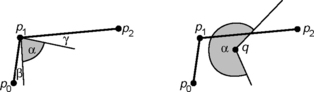
FIGURE 11.7 Neighborhood of p1 (left). Intersection with an uncritical edge (right) [546].
A frontier point can be in a face or on an edge. Suppose first that p1 is in a face f. Either ![]() and f intersect in a straight line segment or f is contained in
and f intersect in a straight line segment or f is contained in ![]() . Intersecting in a straight line segment would contradict the fact that α <Π in the
. Intersecting in a straight line segment would contradict the fact that α <Π in the ![]() 0-neighborhood of p1, and f ⊂
0-neighborhood of p1, and f ⊂![]() would allow p1 to move toward p0p2 in Δ(p0,p1,p2), which contradicts our MLP assumption.
would allow p1 to move toward p0p2 in Δ(p0,p1,p2), which contradicts our MLP assumption.
There are three possibilities for an edge contained in Mρ. We call it uncritical if it is in only one cube contained in ρ; ineffective if it is in exactly two such cubes; and critical (as previously defined) if it is in three such cubes. p1 cannot be on an ineffective edge, and it cannot be on a critical or an uncritical edge, because this corresponds to it being within a face, as discussed before. p1 also cannot be on an uncritical edge or a critical edge.
Figure 11.7 (right) illustrates an intersection q in ![]() with an uncritical edge that is not coplanar with
with an uncritical edge that is not coplanar with ![]() . The angular sector α>Π (the region not in Mρ in an
. The angular sector α>Π (the region not in Mρ in an ![]() -neighborhood of q) does not allow p1 to be such a point. If the uncritical edge were in
-neighborhood of q) does not allow p1 to be such a point. If the uncritical edge were in ![]() ,α would be equal to π, which is also impossible for p1. Thus only one option remains: p1 must be on a critical edge; indeed,α <Π for such an edge.
,α would be equal to π, which is also impossible for p1. Thus only one option remains: p1 must be on a critical edge; indeed,α <Π for such an edge.
Note that this theorem also applies to planar simple 1-curves in [C2, ≤]. It follows that MLP vertices on such a 1-curve can only be convex vertices of the inner frontier or concave vertices of the outer frontier, because these are the only vertices incident with three squares of the 1-curve.
11.1.5 The rubber band algorithm
This algorithm, which is from [148], is based on the following physical model. Suppose a rubber band passes through the tube Mρ. If it can move freely, it will contract to the MLP, which is complete and contained in Mρ, assuming it is smooth enough to slide over the critical edges of the tube.
The algorithm consists of two subprocesses. The first is an initialization process that defines a simple polygonal curve Π0 that is complete and contained in Mρ and such that CΠ0 contains each cube of ρ just once (see Lemma 11.2). The second is an iterative process (a Mρ-transform; see Lemma 11.3) in which each iteration transforms Πt into Πt + 1 (t ≥ 0) such that l (Πt) ≥ l(Πt + 1). Thus the resulting polygon is also complete and contained in ρ.
The following are three methods of initializing the polygon. Init I: The vertices of the initial polygon are at the centers of the cubes that constitute the 2-curve. Init II: The vertices are at the midpoints of critical edges. Init III: The initial polygon connects only vertices that are endpoints of consecutive critical edges.
For Init III, we scan the curve until we find a pair (e0,e1) of consecutive critical edges that are not parallel or (if parallel) that are not in the same grid layer. (Figure 11.6 (right) shows a nonsimple 2-curve; searching for a pair of noncoplanar edges would be insufficient in this case.) For such a pair (e0,e1), we choose vertices (p0,p1), where p0 bounds e0 and p1 bounds e1 such that the line segment p0p1 has minimum length; note that (p0,p1) is not always uniquely defined. This is the first line segment of the initial polygon Π0.
Suppose pi −1 pi is the last line segment on the Π0 specified so far, where pi bounds ei. Then there is a unique vertex pi + 1 on the next critical edge ei + 1 such that pipi + 1 has minimum length. (Length zero is possible if pi + 1 = pi; in this case, we skip pi + 1, which means that we do not increase i.) Note that this pipi + 1 will always be included in the tube, because the centers of all cubes between two consecutive critical edges are collinear. The process stops when we connect pn (on en) with p0. (Note that a minimum-distance criterion for this final step might prefer a line segment between pn and the second vertex bounding e0 [i.e., not p0]). Table 11.1 shows the list of vertices for the curve on the left in Figures 11.6 and 11.8. The first row lists all of the critical edges shown in Figure 11.6. The second row contains the vertices of the initial polygon shown in Figure 11.8 (initialization = first iteration of the algorithm). Vertex b is on edge 2 and also on edge 3, so there is only one column (2/3) for these edges.
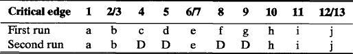

FIGURE 11.8 Curve initializations (Init III; “clockwise”) [149].
Initialization methods Init I through Init III construct polygons Π0 that are always complete and contained in the given tube. Note that traversals in opposite directions or that start at different critical edges may lead to different initial polygons if Init III is used. For example, a “counterclockwise” traversal of the curve shown in Figure 11.6 (left) starting at edge 1 selects edges 11 and 10 as the first pair of consecutive critical edges; the resulting “counterclockwise” polygon differs from the one shown in Figure 11.8. Figure 11.9 shows a curve for which the final step does not return to the starting vertex.

FIGURE 11.9 If the initialization starts below on the left, the final step of the initialization process would prefer the second vertex of the first edge [149].
The results of Init III are shown in Figure 11.8. The curve on the right is already an MLP for this nonsimple 2-curve. For a planar curve, the process may fail to find the first pair of critical edges; in this case, a 2D algorithm can be used to calculate the MLP.
In the iteration process, we move pointers (addressing three consecutive vertices of the polygonal curve found so far) around the curve until a complete iteration leads only to an improvement that is below a given threshold τ (i.e.,l(Πt) –τ < l(Πt + 1)). We cannot wait until there is no change at all, because this may never happen. In all of the experiments reported in [149], the algorithm terminated quickly for a reasonable value of τ.
Let Πt =(p0,p1,…,pm) be a polygon with three pointers addressing the vertices at positions i −1, i, and i + 1. Three cases can occur that define specific Mρ-transforms.
(O1) pi can be deleted iff pi + 1 pi + 1 is a line segment within the tube. Triple (pi−1,Pi,Pi + 1) is then replaced by (pi−1,pi + 1), and we continue with vertices pi−1, pi + 1,and pi + 2.
(O2) The closed triangular region Δ(pi−1 pipi + 1) intersects more than just the three critical edges of pi−1, pi, and pi + 1 (see Figure 11.10) (i.e., simple deletion of pi would not be sufficient). This situation is handled by constructing a convex arc (the shortest curve that surrounds a given finite set of planar points is a convex polygon [155]) and replacing pi with the sequence of vertices q1,…,qk between pi−1 and pi + 1 on this arc iff the sequence of line segments pi−1 q1,…,qkpi + 1 lies inside the tube. Because the vertices are ordered, we can use a linear-time convex hull algorithm. Barycentric coordinates with basis {pi−1,pi,pi + 1} can be used to decide which of the intersection points are inside the triangle.1 In this case, we continue with a triple of vertices that starts with qk.
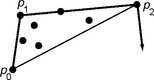
FIGURE 11.10 Intersection points with edges [149].
(O3) pi can be moved on its critical edge to a position pnew that minimizes the total length of pi−1pnew and pnewpi + 1. An O(1) algorithm for this move is given below. (pi−1,pi,pi + 1) is then replaced by (pi−1,pnew,pi + 1), and we continue with the triple p new, pi + 1,pi + 2.
In situation (O3), suppose pi lies on critical edge e and is not collinear with pi−1pi + 1. Let le be the line containing e. We first find the point popt ∈ le such that the following is true,
and where we also have the following:
If popt lies on the closed critical edge e, we simply replace pi with popt; if not, we replace pi with the vertex bounding e that lies closest to popt.
The following is a slightly simpler method of finding popt than the one described in [148]. Without loss of generality assume that le is parallel to the x-axis, where ye and ze are constants:
If xi−1 = xi + 1, we take popt = (xi−1,ye,ze)T. Otherwise, the following
leads to a quadratic equation in xopt, where αi = (ye – yi)2 + (ze – zi)2:
Table 11.1 shows that the second run starts with the polygonal curve Π1 = (a,b,c,d,e,f,g,h,i,j). For triple a,b,c, none of (O1) through (O3) leads to a better location of b. For triple b, c, d, we use (O1) to delete c (symbol ‘D’). Triple b, d, e then leads to the deletion of d, and so on, and finally triple j, a, b does not delete or move a. In the following run, nothing changes.
The process stops if an entire cycle does not lead to a “significant modification” as defined by a threshold τ.2 Experiments in [149] used τ s between l (Πt)·10−5 and l(Πt) · 10−7. In Figure 11.11, the initial polygon Π0 is dashed, and the solid line is the final polygon. The short line segments are the critical edges of the tube.

FIGURE 11.11 Two examples of initial polygons (dashed) and MLPs (solid). Critical edges are shown as short line segments. The rest of the tube is not shown [149].
We conclude this section by giving an estimate of the complexity of the rubber-band algorithm as a function of the number n of cubes of ρ.
The algorithm completes each run in O(n) time. A move of pi on a critical edge requires constant time. In the experiments,τ was set to l(Π0) · 10−6; this ensured that the measured time complexity was O (n) (i.e., the number of runs did not depend on n).
Figure 11.12 shows the time needed for the algorithm to stop as a function of the number of cubes n and the number of critical edges. The test set contained 70 randomly generated simple 2-curves. In Figure 11.12 (left), each error bar shows the mean convergence time and its standard deviation for a set of 10 digital curves.
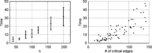
FIGURE 11.12 Central Process Utility (CPU) time in seconds as a function of the number n of 3-cells (left) and the number of critical edges (right) [149].
The algorithm is iterative. Because l(Πt + 1) < l (Πt) (if they are equal, the algorithm stops) and there is a lower bound on the length 1(Πt) of the MLP, the algorithm converges. However, it is not certain to what polygon it converges. Lemmas 11.2 and 11.3 give a partial answer: it always converges to a polygon that is complete and contained in Mρ.
The algorithm provides a method of polygonal approximation and length measurement of simple 2-curves that has run time O(n). The method has been successfully used for a wider class of curves, including cases such as the curve on the right in
Figure 11.6 in which each cube in ρ has exactly two bounding faces in ρ. This simpler definition also allows for the simpler generation of test examples.
It would be desirable to prove that the time complexity of the algorithm is always O(n) and that it always converges to the MLP. Both of these statements can be conjectured from the experiments: the number of cycles was independent of the resolution of the 2-curve, and the minima found by the algorithm were independent of the initialization method.
11.2 Digital Planes in 3D Adjacency Grids
A plane in E3 that has a z-coefficient that is not 0 is defined by an expression of the following form, where α1,α2,β ∈ R:
The symmetry of the grid allows us to assume 0 ≤α1 ≤ 1 and 0 ≤α2 ≤ 1 in the rest of this chapter; we also assume 0 ≤β < 1 for convenience, using an argument similar to that for DSLs.
A digital plane can be obtained from a plane in E3 by outer 3D Jordan digitization, 3D grid-line intersection digitization (using the grid points nearest to the intersections of the plane with grid lines; compare the 3D grid-plane intersection digitization in Section 11.1.1), or simply by applying the floor or ceiling function to the coordinates of the points in Γ(α1,α2,β).
11.2.1 3D grid-line intersection digitization
If we use 3D grid-line intersection digitization, under the above assumptions about α1,α2,β, we need to consider only grid lines parallel to the z-axis.
Let Γ(α1α2,β) intersect the vertical grid line (x = m,y = n)at pm,n where m,n ≥ 0. Then the grid point closest to pm,n is (m,n,Im,n) where the following is true:
If there are two closest grid points, we choose the lower one. The set Iα1,α2,β uniquely determines both the slopes α1 and α2 and the intercept β if α1 or α2 is irrational. If both α1 and α2 are rational, Iα1,α2,× uniquely determines α1 and α2 but determines β only up to an interval. This can be proved by a straightforward generalization of the proof of Theorem 9.2
In analogy with the chain codes in Chapter 9, we define step codes, starting with iα1,α2,β(0,0) = I0,0 ∈{0,1}:

In addition to these “initial values,” we define column-wise step codes:

We also define row-wise step codes:
The values in the 0th row and 0th column are used in both the column-wise and rowwise step codes; see Figure 11.13. The assumptions 0 ≤α1 ≤ 1 and 0 ≤α2 ≤ 1 guarantee that codes 0 and 1 are sufficient. It follows that ![]() where m,n ≥ 0. On the basis of the additional assumption α1 ≤α2, we will use only row-wise step codes in the sequel, and we will omit the superscript (r).
where m,n ≥ 0. On the basis of the additional assumption α1 ≤α2, we will use only row-wise step codes in the sequel, and we will omit the superscript (r).

FIGURE 11.13 Left: ![]() . Middle:
. Middle: ![]() . Right:
. Right:![]() (m,n) [131].
(m,n) [131].
Definition 11.2
![]() is a digital plane quadrant (in the grid point model) with slopes α1 and α2 and intercept β.
is a digital plane quadrant (in the grid point model) with slopes α1 and α2 and intercept β.
If we do not require m and n to be nonnegative integers, we obtain digital planes iα1,α2,β. For D ⊇ R, let ![]() . If α1 or α2 is irrational, we speak about irrational digital planes and otherwise about rational digital planes.
. If α1 or α2 is irrational, we speak about irrational digital planes and otherwise about rational digital planes.
Analogously to the translation-equivalence of rational DSLSs with the same slope α [675], we have translation-equivalence of rational digital planes with the same slopes α1 and α2 [134]. This implies that the intercepts β do not influence translation-invariant properties of rational digital straight lines; we can therefore study translation-equivalence classes iα1,α2 of rational digital planes.
Using Definition 7.5 of digital surfaces (and digital surface patches) in adjacency grids, we have the following:
11.2.2 Self-similarity
Obviously, a simple digital surface that satisfies the chordal property cannot be bounded.
Defining evenness with respect to the xy-plane is consistent with our previous assumptions about digital planes. By requiring a one-to-one mapping into the xy-plane, we consider only unbounded sets S ⊆ Z3 as being even. The following theorem does not make use of the assumption α1 ≤α2 about a digital plane.
11.2.3 Supporting and separating planes
A supporting plane of S ⊆ Z3 divides R3 into two (closed) halfspaces such that S is completely contained in one of them.
Theorem 11.8
S ⊆ Z3 is a digital plane iff it has a supporting plane Γ such that the L∞-Hausdorff distance between S and Γ is < 1.
In [513], it was claimed that if S ⊆ Z3 is a (finite) digital plane segment, the points of S are at L∞-Hausdorff distance < 1 from at least one plane incident with one of the faces of the convex hull of S; thus one of these planes is a supporting plane in the sense of Theorem 11.8. However, [253] gave a counterexample: if D = [0,6]× [0,7], the L∞-Hausdorff distance between ![]() and any plane incident with one of the faces of the convex hull of
and any plane incident with one of the faces of the convex hull of ![]() is greater than 1.
is greater than 1.
Let S ⊂ Z3, and let Sz + 1 = {(x,y,z + 1):(x,y,z) ∈ S}. A plane Γ ⊂ R3 separates the sets S1,S2 ⊂ Z3 iff S1 and S2 are in opposite open halfspaces defined by Γ.
11.2.4 Arithmetic planes
Arithmetic geometry as suggested by S. Forchhammer in [332] and developed by J.-P. Reveill ès in [848] provides a uniform approach to the study of digitized hyperplanes in n dimensions. We discuss here only the 3D case. Let a, b, and c be relatively prime integers, and let μ and ω be integers.
Arithmetic planes are a generalization of arithmetic lines Da,b,μ,ω= ∈ Z2 :μ ≤ ai + bj <μ +ω}. From Theorem 9.4, we know that naive lines (ω = max{|a|, |b|}) are the same as rational DSSs and that standard lines (ω = |a| + |b|) are the same as rational 4-DSSs. If ω = max{|a|, |b|, |c|}, the arithmetic plane Da,b,c,μ,ω is called a naive digital plane; if ω = |a| + |b| + |c|, it is called a standard plane.
In other words, for any digital plane iα1,α2,β with rational α1 and α2, there exist relatively prime integers a, b, and c and an integer μ such that iα1,α2,β = Da,b,c,μ,max{|a|,|b|,|c|}. In addition, for any Da,b,c,μ,max{|a|,|b|,|c|}, there exist rational slopes α1 and α2 and an intercept β such that Da,b,c,μ,max{|a|,|b|,|c|} = iα1,α2,β.
Now assume 0 < a≤ b ≤ c, and consider digitizations of Euclidean planes that are incident with the origin (e.g., by assuming μ = 0). If Da,b,c,0,ω is a naive plane, each voxel (x,y,z) ∈ Da,b,c,0,c projects into exactly one pixel (x,y) in the xy-plane. From the assumption 0 < a≤ b ≤ c, it follows that there is at least one voxel (x,y,z) ∈ Da,b,c,0,ω for every (x, y) ∈ Z2.The height map Ha,b,c,ω is defined on Z2 by assigning the maximum value z to (x,y) such that (x,y,z) ∈ Da,b,c,0,ω.
Figure 11.14 illustrates two height maps of naive planes Da,b,c,0,c. Let La,b,c(z0) = {(x,y) ∈ Z2 :(x,y,z0) ∈ Da,b,c,0,c} where z0 ∈ Z. Then La, b,c(z0) is an arithmetic line D(a,b,μ,ω) with μ = −cz0 and ω = c. D(a,b,μ,ω) is standard if c = a + b, “thicker than standard” if c > a + b, and “thinner than standard” but “thicker than naive” if c <a + b. The arithmetic lines La,b,c(z0) with z0 ∈ Z partition Z2 into equivalence classes that are all translation equivalent3 iff a and b are relatively prime [134]. Figure 11.14 shows height maps for a case in which a and b are relatively prime (left) and a case in which they are not relatively prime (right).

FIGURE 11.14 Height maps: D67,16,0,16 on the left; D6,9,16,0,16 on the right [134].
0 < a ≤ b ≤ c implies that the projections ![]() (where x0,y0 ∈ Z) are naive lines with approximate intercepts μ = − ax0 and μ = − by0, respectively. The arithmetic lines
(where x0,y0 ∈ Z) are naive lines with approximate intercepts μ = − ax0 and μ = − by0, respectively. The arithmetic lines ![]() , where x0 ∈ Z, partition Z2 into translation-equivalent equivalence classes. The same is true for the arithmetic lines
, where x0 ∈ Z, partition Z2 into translation-equivalent equivalence classes. The same is true for the arithmetic lines ![]() for y0 ∈ Z; see [253, 255].
for y0 ∈ Z; see [253, 255].
Naive planes can also be represented by arrays of remainders [253]. Let (x,y,z) ∈ Da,b,c,0,c. We assign value ax + by + cz to grid point (x,y) (i.e., its remainder modulo c). This results in a remainder map Ra,b,c. Figure 11.15 shows two examples. On the left, we have a = 6 and b = 7 (i.e., the integers are relatively prime, which results in remainders in the entire range 0,…, 15 for c = 16). On the right, we have a = 6 and b = 9 (i.e., the remainders in each equivalence class of the depth map are all equal modulo gcd(6,9) = 3).

FIGURE 11.15 Remainder maps for the naive planes shown in Figure 11.14 [134].
11.2.5 Periodicity
A position (i,j) in an array X = (X(i, j))0≤i 0≤j is defined by a row i and a column j; X(i,j) is the element of X at position (i, j). The elements of X are letters in an alphabet A. We continue to assume 0 ≤α1,α2 ≤ 1; hence, in a digital plane quadrant, we have A = {0,1}.
Let ![]() . The restriction X[S] of X to positions in S is called a factor of X on S.
. The restriction X[S] of X to positions in S is called a factor of X on S.
An infinite array X on ![]() is called 2D-periodic iff there are two linearly independent vectors u and v in Z2 such that w = iu + jv is a period for X for any (i, j)∈ Z2 and
is called 2D-periodic iff there are two linearly independent vectors u and v in Z2 such that w = iu + jv is a period for X for any (i, j)∈ Z2 and ![]() . X is called 1D-periodic iff all periods of X are parallel vectors.
. X is called 1D-periodic iff all periods of X are parallel vectors.
Let X be a 2D-periodic infinite array on ![]() . The set of symmetry vectors of X defines (by additive closure) a subgrid Λ of Z2. Any basis of Λ is a basis of X.
. The set of symmetry vectors of X defines (by additive closure) a subgrid Λ of Z2. Any basis of Λ is a basis of X.
We say that an infinite array X on ![]() is tiled by a (finite) rectangular factor W if X is a pairwise disjoint repetition of W. Evidently, any 2D-periodic array on
is tiled by a (finite) rectangular factor W if X is a pairwise disjoint repetition of W. Evidently, any 2D-periodic array on ![]() can be tiled.
can be tiled.
Theorem 11.12
The lattice cells of all bases of a rational digital plane quadrant have constant area max{|a|,|b|,|c|}.
Let X be an array on ![]() . An m × n
. An m × n ![]() defines an m × n-factor of X. Any rectangular factor of an irrational digital plane is also a factor of a rational plane.
defines an m × n-factor of X. Any rectangular factor of an irrational digital plane is also a factor of a rational plane.
Let PX (m, n) be the number of m × n-factors of X. For example, PX (0,0) = 1 for any X, and PX (1,1) is the number of distinct letters in X. (In our case, A = {0,1}.) PX generalizes the complexity function P(w,n) defined in Chapter 9.
An array X on ![]() is called Sturmian iff it is an infinite array of an irrational digital plane where both slopes,α1 and α2, are irrational numbers. The height h(W) of an m × n array W is the number of 1s in W. If V and W are of the same size,δ(V,W) = | h(V) – h(W) | is called their balance. A set of arrays X of identical size is called balanced iff δ(V,W) ≤ 1 for all pairs V, W of the arrays. An infinite array X on
is called Sturmian iff it is an infinite array of an irrational digital plane where both slopes,α1 and α2, are irrational numbers. The height h(W) of an m × n array W is the number of 1s in W. If V and W are of the same size,δ(V,W) = | h(V) – h(W) | is called their balance. A set of arrays X of identical size is called balanced iff δ(V,W) ≤ 1 for all pairs V, W of the arrays. An infinite array X on ![]() is called array!balanced iff its set of m × n-factors is balanced. An array X on
is called array!balanced iff its set of m × n-factors is balanced. An array X on ![]() is called eventually periodic iff there exist integers k and l such that the array (X(i, j))k ≤ i, i≤j (which is a suffix of X) is periodic.
is called eventually periodic iff there exist integers k and l such that the array (X(i, j))k ≤ i, i≤j (which is a suffix of X) is periodic.
11.2.6 Connectivity of arithmetic planes
An arithmetic line becomes 8-disconnected iff ω < max{|a|, | b|}. Similarly, an arithmetic plane Da,b,c,μ,ω no longer has grid points on all of the vertical grid lines iff ω < max{|a|, |b|, |c|}.
A standard arithmetic plane is 26-separating and gapfree; it has no 6-, 18-, or 26-gaps. A naive arithmetic plane is 6-separating but not necessarily 18- or 26-separating; it can have 18- or 26-gaps. Note that, if S is not α-connected, any of its subsets is α-separating in S.
In Chapter 9, we formulated equivalences between 8-gap-freeness and 4-connectedness (4-gap-freeness and 8-connectedness) for arithmetic lines; this cannot be done for arithmetic planes. Connectivity is a translation-invariant property. Without loss of generality, we consider grid-line intersection digitizations of rational planes ax + by + cz = 0 that are incident with the origin. Let Da,b,c,ω be the corresponding arithmetic plane with thickness ω ∈ Z+ where a,b,c ∈ Z and gcd(a,b,c) = 1. In the case of a naive plane (ω = max{|a|, |b|,|c|}), we simply write Da,b,c.
ω = Ωα(a, b, c) + 1 is the smallest integer such that Da,b,c,0,ω is α-connected. Evidently,α ≥β (α,β ∈{6,18,26}) implies Ωα(a,b,c) ≤Ωβ(a,b,c). Naive planes are always 26-connected (i.e., Ω26(A,b,c) ≤ max{|a|,|b|,|c|}), and standard planes are always 6-connected (i.e., Ω6(a, b, c) ≤|a| + |b| + |c|). Connectivity numbers remain unchanged when a, b, and c are permuted (e.g., Ωα, (a,b,c) = Ωα, (b,c,a)).
Exercise 7 in Section 11.5 defines “jumps” and shows that they exist in naive planes if c <a + b. Figure 11.16 illustrates such a naive plane in which 8-connected sets of pixels in the height map may be projections of 26-disconnected sets of voxels in the plane. The Symmetry Lemma (Proposition 11.1) allows us to transform such naive planes into symmetric (in the sense of the Lemma) naive planes for which c <a + b is no longer true. This implies the following:
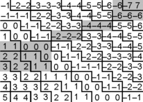
FIGURE 11.16 Height map of the naive plane D5, 7,11,0,11. The 8-connected set of pixels (shown in gray) is a projection of a 26-disconnected set of voxels of this plane [134].
Theorem 11.15
Let a, b, and c be relatively prime integers such that c ≥ a + 2b and a > 0. Then Ω26(a,b,c) = c – a – b + gcd(a,b) − 1.
This theorem, combined with Proposition 11.2, allows us to derive other solutions, such as the following:

Theorem 11.16
If a + b <c <a + 2b, then a − 1 ≤Ω26(a,b,c) ≤ b − 1.
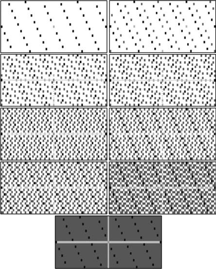
A more instructive understanding of the the plane connectivity issue can be obtained by generating remainder maps Ma,b,c for thicknesses ω in the range from 0 to c. The patterns in Figure 11.17 visualize the pixels that belong to M11,19,35 for ω = 1, 2, 6, 7, 11, 12, 13, 20, and 35. We have Ω26(11,19,35) = 12. By varying the parameters a, b, c, and ω, we can calculate a family of patterns, some of which have interesting (local or recursive) configurations. Studying their properties might be of interest for studying tilings of the plane.
11.3 Digital Planes in the 3D Incidence Grid
A cellular digital plane can be defined by considering a digital plane (or naive plane) in the grid cell model. It can also be defined by outer Jordan digitization of a plane Γ in the grid cell model. However, if Γ passes through a grid vertex or contains a grid edge, outer Jordan digitization produces “locally thicker” cellular planes.
The frontier of a cellular digital plane consists of two “parallel layers” of frontier faces that define an upper and a lower digital frontier plane in the incidence grid C3; they are analogous to the lower and upper digital rays or lines defined in Chapter 9.
Each 0-cell of a 3-cell c is incident with three 2-cells of c. The normals to these 2-cells form a tripod, and there are eight different tripods. All of the face normals of any upper or lower digital frontier plane belong to one tripod.
Definition 11.8
![]() is called a digital plane of 2-cells in the incidence grid iff it is an upper or lower digital frontier plane defined by a cellular digital plane.
is called a digital plane of 2-cells in the incidence grid iff it is an upper or lower digital frontier plane defined by a cellular digital plane.
A finite 1-connected subset of a digital plane of 2-cells is called a digital plane segment (DPS) in the 3D incidence grid.
In the plane (see Theorem 9.5), a 4-path is a 4-DSS iff it is contained between or on a pair of supporting lines with a main diagonal distance of less than ![]() . Let G be a finite 1-connected set of faces of grid cubes. Let the faces be contained between or on a pair of parallel planes. The main diagonal v =(±1, ±1, ±1) of a pair of parallel planes is the diagonal direction (one of the eight possible directed diagonals in the 3D grid with length
. Let G be a finite 1-connected set of faces of grid cubes. Let the faces be contained between or on a pair of parallel planes. The main diagonal v =(±1, ±1, ±1) of a pair of parallel planes is the diagonal direction (one of the eight possible directed diagonals in the 3D grid with length ![]() ) that has the greatest dot product (inner product), with the outward pointing normal n to the planes. If there is more than one such direction, we can choose one of them arbitrarily. The distance between the planes in the main diagonal direction is called their main diagonal distance.
) that has the greatest dot product (inner product), with the outward pointing normal n to the planes. If there is more than one such direction, we can choose one of them arbitrarily. The distance between the planes in the main diagonal direction is called their main diagonal distance.
Proposition 11.3
A finite 1-connected set of frontier faces of a set of 3-cells is a DPS iff all of the face normals belong to one tripod and the faces are contained between or on a pair of parallel planes with a main diagonal distance of less than ![]() .
.
In other words, a DPS in the incidence grid can be assumed to be a 1-connected set of 2-cells in the frontier of a 6-region of voxels. If considered together with its incident 0- and 1-cells, it is a 2D Euclidean cell complex. A simply connected DPS consists of faces that have a union that is homeomorphic to the unit disk (i.e., it is a 1- simply connected set of 2-cells). Figure 11.18 shows a DPS; n is its normal, and v is the vector in the main diagonal direction.

If we are given the frontier of the projection of the DPS onto one of the two parallel planes, it is possible to reconstruct the DPS in 3D space (up to a translation in the normal direction to the planes).
Let v be the vector of length ![]() in main diagonal direction, and let n be an outward pointing normal to the pair of parallel planes. Let p be a grid vertex incident with the DPS, and let v · p = dp be the equation of a plane incident with p that has normal v. In accordance with Proposition 11.3, the vertices p of the grid faces of a DPS must satisfy the following:
in main diagonal direction, and let n be an outward pointing normal to the pair of parallel planes. Let p be a grid vertex incident with the DPS, and let v · p = dp be the equation of a plane incident with p that has normal v. In accordance with Proposition 11.3, the vertices p of the grid faces of a DPS must satisfy the following:
Let n =(a, b, c). The scalars a, b, and c can have different signs, but, because n and v must point in the same direction “modulo a directed diagonal,” we can assume without loss of generality that a,b,c > 0.Equation 11.5 then becomes the following:
Hence, a DPS in the grid-cell model is equivalent (by mapping vertices into grid points) to a finite 6-connected set of grid points in a standard digital plane (see Definition 11.5) for which v = dp and ω = a + b + c.
In addition to checking the tripod condition (which is easy), DPS recognition (in the grid cell model) can be performed by answering the following question: Given n vertices {p1,p2,…,pn}, does each pi such that di = v · pi satisfy Equation 11.5? Or, to put it another way, do we have the following?
11.4 DPS Recognition and Generation
Theorem 11.9 was used in [1028] to suggest a DPS recognition algorithm based on convex hull separability. The recognition of DPSs in grid-adjacency models (i.e., DPSs regarded as subsets of Z3) is also discussed in [1089] (using the characterization by evenness given previously), [549] (using least-square optimization), and [157,716, 823, 1100] (using linear programming). [255] discusses the use of arithmetic “limits.” ax + by + cz = μ and ax + by + cz = μ +ω are called the lower and upper supporting planes of an arithmetic plane; a test for the existence of these planes provides another method of designing algorithms for DPS recognition. Supporting planes are called leaning planes in arithmetic geometry.
[341] suggests a method of recognizing DPSs in the incidence grid based on conversion of Equation 11.5 into a system of linear inequalities by eliminating the
This system of n2 inequalities can be solved in various ways. [341, 340] uses the Fourier-Motzkin algorithm. We can also use Fukuda ’s cdd algorithm4 for solving systems of linear inequalities by successive intersection of halfspaces defined by the inequalities.
11.4.1 An incremental DPS algorithm
We will next describe an incremental algorithm [550]. Typical timing results for these three algorithms are shown in Figure 11.19 for a polyhedrized digital ellipsoid at grid resolutions ranging from 10 to 100.
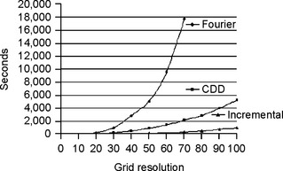
FIGURE 11.19 Running times of three DPS recognition algorithms on a PIII 450 running Linux. (Laurent Papier provided the Fourier-Motzkin program.)
Algorithm KS2001
Π is called a supporting plane of a finite set of faces if the faces are all in one of the closed halfspaces defined by Π and their diagonal distances to Π are all less than ![]() . If the set of faces has n ≥ 4 vertices, Π must be incident with three noncollinear vertices, and all the other vertices must lie on or on one side of Π. A set of faces can have more than one supporting plane.
. If the set of faces has n ≥ 4 vertices, Π must be incident with three noncollinear vertices, and all the other vertices must lie on or on one side of Π. A set of faces can have more than one supporting plane.
The incremental algorithm repeatedly updates a list of supporting planes; if this list is empty, the set of points is not a DPS. The updating step is as follows: if we have n ≥ 0 points, we add an (n + 1)st point iff the list of supporting planes remains nonempty. To test this, we first check the new point against each of the listed supporting planes to see if it is on the same side of the plane as the other points and within the allowed diagonal distance. We delete the plane from the list if these conditions are not satisfied. We then construct new supporting planes by combining the new point with pairs of existing points. A new supporting plane is added to the list if all n + 1 points satisfy the conditions. The set of points is accepted as a DPS iff the final list of planes is not empty. The updating step is time-efficient, because we can restrict the tests to points that have extreme positions in any of the eight diagonal directions.
A surface consists of edge-connected faces. These faces can be represented by a face graph that has nodes that are the faces and in which each node has four pointers to its edge-adjacent faces. The face graph can be constructed using, for example, the Artzy-Herman surface tracing algorithm.
We can perform a breadth-first search of the face graph to agglomerate the faces into DPSs. This process is implemented using two queues. The first is called a seeds queue; it contains all of the faces found by the search that do not belong to any yet recognized DPS. A face is inserted into the seeds queue if it cannot be added to the current DPS. The next DPS starts from a face chosen from the seeds queue; the choice of this face determines how the DPS “grows.” The second queue is used to maintain the breadth-first search. “Growing a DPS” looks like propagating a “circular wave” on the surface from a center at the original seed face.
We try to add an adjacent face to the current DPS by testing each vertex of the face that is not yet on the DPS. If all four vertices pass the test, the face is added to the DPS and deleted from the seeds queue (if it was on that queue). Otherwise, we insert the face into the seeds queue and try another adjacent face. If no more adjacent faces can be added, we start a new DPS from a face on the seeds queue.
A list of the frontier vertices of each DPS is maintained during the agglomeration process, not only to simplify the tests for whether a new vertex can be added but also to maintain the topologic equivalence of the DPS to a unit disk. This ensures that the frontier always remains a simple polygon so that the algorithm constructs only simply connected DPSs. (This condition can be removed, if desired.)
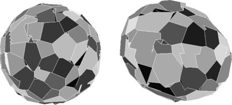
Figure 11.20 illustrates results of the agglomeration process for a digitized sphere and for an ellipsoid with semiaxes 20, 16, and 12. Faces that have the same gray level belong to the same DPS. The numbers of faces of the digital surfaces of the sphere and ellipsoid are 7584 and 4744, respectively. The numbers of DPSs are 285 and 197; the average sizes of these DPSs are 27 and 24 (faces).

FIGURE 11.20 Agglomeration into DPSs of the faces of a sphere and an ellipsoid (with a grid resolution of h = 40).
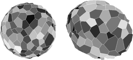
To complete the polyhedrization process we take all of the face vertices that are incident with at least three of the DPSs as the vertices of the polyhedron. Figure 11.21 shows the final polyhedra for the sphere and ellipsoid. Note that these polyhedra are not simple; their surfaces are not hole-free.
Restricting the depth of the breadth-first search changes the polyhedrization from global to local and results in “more uniform” polyhedra. Figure 11.22 shows results when the depth is restricted to 7. The number of small DPSs is reduced, and the sizes of the DPSs are more evenly distributed. The numbers of DPSs are 282 and 180, and their average sizes are 27 and 26; note that these are nearly the same as in the unrestricted case.
11.4.2 DPS generation algorithms
Consider the task of obtaining a gap-free digitization of the surface of a simple polyhedron “face-by-face.” If every polygonal patch on the surface of the polyhedron is approximated (digitized) individually (!) by a naive plane, gaps may result “near the edges” of the polyhedron.
A method from [62] for solving this problem is based on reducing the 3D problem to a 2D one by projecting the polygonal patches onto suitable coordinate planes, digitizing the resulting 2D polygons (in the thinnest way possible, in the terminology of arithmetic geometry), and then finally calculating the 3D digital polygons as subsets of naive planes.
Another method [135] approximates every 3D polygon by a digital polygon, again in the thinnest way possible, and approximating the edges of the polygons by 3D DSSs. The resulting digitization is “optimally thin” in the sense that removing any voxel from the digital surface produces a gap. A third method [133] is based on using graceful planes and lines, respectively, to approximate the surface polygons and their edges. The algorithms in the cited references run in times that are linear in the number of generated surface voxels.
11.5 Exercises
1. Prove statements 11.1 through 11.4.
2. If the projections of a 26-DSS are an 8-DSS with normal (x1,x2) in the (x = 0)-plane and an 8-DSS with normal (y1,y2) in the (y = 0)-plane, what is the normal of the 26-DSS?
3. Generate the following circles γ(t) in R3, where Rx and Rz are 3 × 3 matrices of rotations around the x- and z-axes, respectively:

The angles η1,η2, and η3 and the radius r are randomly chosen from uniform distributions in [0,2π) and [0.5,1], respectively. Perform grid-plane intersection digitization of each generated circle using varying grid sizes (e.g., between 1003 and 10003). Implement 3D DSS segmentation and 3D MLP approximation, and compare their run times.
4. (Open problem) Is there a simple 2-curve such that none of the vertices of its 3D MLP is a grid vertex (i.e., none of these vertices is an endpoint of a critical edge)?
5. Give an example of a 2-curve with a 3D MLP that has at least one vertex that has an irrational coordinate.
6. A straight line in 3D space can be represented as the intersection of two planes aix + biy + cic + d1 = 0(i = 1,2). Give an example in which the intersection of two digital planes (i.e., two naive planes) obtained by grid-line intersection digitization of two distinct planes is 26-disconnected.
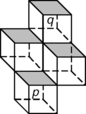
7. Two voxels p = (i,j, k) and q = (i + 1, j + 1, k + 2) in the grid cell model (see the following figure) define a jump. Show that a naive plane Da,b,c,μ,c (where c = max{a, b,c}) has a jump iff c <a + b.
8. There are four possible factors of size 2 × 2 of a digital plane quadrant for which 0 ≤α1,α2 ≤ 1, and α1 ≤α2. Which pairs of these factors can be contained in the same rational digital plane quadrant?
9. Prove that a rational digital plane quadrant has at most mn distinct factors of size m × n.
10. Implement algorithm KS2001 and test it on digitized ellipsoids with varying semiaxes 0 < a,b,c ≤ 1 for different grid resolutions, for example, h = 100,…,1000. Study the impact of different search strategies and search depth thresholds on the run time and on the resulting DPS segmentation.
11. Design a DPS approximation algorithm along the following lines: incrementally calculate the 3D convex hull of a set of grid points to which one 6-connected grid point is added at a time, and incrementally update the minimum width of the convex hull as long as the minimum width is below a predefined threshold (e.g., ![]() or larger, allowing for “minor variations”).
or larger, allowing for “minor variations”).
12. Prove that the connectivity number Ω26 satisfies (i) Ω26 (a, a, a) = 0, (ii) Ω26 (0,b,c) = c − 1, (iii) Ω26(a,b,b)= b − 1, (iv) Ω26(a,a,c) = c – a − 1, and (v) Ω26(a,b,2b) = b − 1, where a, b, and c are relatively prime integers such that 0 < a ≤ b ≤ c.
11.6 Commented Bibliography
For reviews of 3D straight lines, see [210] (in computer graphics) and [480] (in 3D picture analysis).
Theorem 11.1 is from [511]; for a generalization to straight lines in Zn, see [540]. The digitization of hyperplanes in arbitrary dimensions is discussed in [540].
[325] defines 3D DSSs in arithmetic geometry using Diophantine inequalities. A more specific definition is given in [203] for the purpose of deriving an efficient 3D DSS recognition algorithm. Sections 11.1.2 and 11.1.3 review parts of [203]. Theorem 11.3 is proved in [253]; see also [256].
Algorithm DR1995 is used in [203] to recognize 26-DSSs (see Section 11.1) and to estimate the lengths of 3D curves; see Chapter 12 for estimation results.
A brief description of the iterative 3D MLP algorithm and some preliminary experimental results were presented in [148]. The difficulty of the subject is illustrated by the fact that the Euclidean shortest path problem (given a finite collection of polyhedral obstacles in 3D space and a source and a target point, find a shortest obstacle-avoiding path from source to target) is known to be NP-hard [162]. However, there are polynomial-time algorithms for the approximate Euclidean shortest path problem; see [198]. The convergence behavior of the algorithm in [148] is not yet known; it may converge to the exact 3D MLP, or it may approximate it up to some error. Experiments performed so far suggest that the algorithm always converges to the correct 3D MLP, and time measurements support the hypothesis that its runtime behavior is asymptotically linear in the number of input 3-cells, even if a very small threshold is used for termination.
[171] describes an algorithm for estimating 3D straight lines based on projections onto a plane.
Row- and column-wise step codes of digital planes were introduced in [129]. For the recognition of digital planes, see [519]; for the recognition of digital naive planes, see [1099, 1100]. For the approximation of linear and affine functions, see [866, 871]. For arithmetic straight lines and planes, see [341].
Theorems 11.5 and 11.6 are from [513]. Definition 11.3 is from [517]. Evenness of digital arcs was studied in [454] and generalized in [1088] to evenness of sets in Zn. Theorem 11.7 is proved in [1088].
For the definition of supporting planes and Theorem 11.8, see [513]. Theorem 11.9 is from [1028], where it is proved for digitized hyperplanes of any dimension.
An arithmetic representation of digital planes was introduced in [332]. For a study of digitized hyperplanes of arbitrary dimension based on pairs of Diophantine inequalities, see [23]. Definition 11.5 and Theorem 11.10 are from [848]. For Theorem 11.14, see [23], which actually discusses the general n-dimensional case:
Theorem 11.17
Let ![]() be a digital hyperplane, where b ≥ 0, ai ≥ 0 for all i and ai ≤ ai + 1 for 1 ≤ i ≤ n −1. Then, if ω < an, the digital hyperplane has (n − 1)-gaps. For 0 < k < n,if
be a digital hyperplane, where b ≥ 0, ai ≥ 0 for all i and ai ≤ ai + 1 for 1 ≤ i ≤ n −1. Then, if ω < an, the digital hyperplane has (n − 1)-gaps. For 0 < k < n,if ![]() the digital hyperplane has (k − 1)-gaps and is k-separating. If
the digital hyperplane has (k − 1)-gaps and is k-separating. If ![]() , the digital hyperplane is gapfree.
, the digital hyperplane is gapfree.
This theorem answers the question about the maximal thickness ω for which α-gaps appear. Analytic definitions of digital hyperplanes can also be based on real parameters b,a1,…,an; this allows us to characterize digital planes that have irrational slopes (compare Theorem 11.10) with arithmetic planes defined by at least one irrational parameter.
In [129], V.E. Brimkov extended periodicity studies in the theory of words (Chapter 9) to 2D words based on [18, 351]. Section 11.2.5 briefly reviews his work. [849] proves that PX (m,n) ≤ mn if X is a rational digital plane quadrant (see Exercise 9). Section 11.2.6 reviews [134]. This report also gives an algorithm for computing Ω26(a,b,c), which has a runtime (measured in arithmetic operations) that is O(a log b).
The incremental algorithm KS2001 in Section 11.4, including its derivation and experimental results, was published in [550]. See also [796] for polyhedrization algorithms.
Exercise 3 describes an experiment reported in [149]. For Exercise 6, see [62, 255]. Exercise 7 is from [133]. For Exercise 12, see [134].
1In the majority of cases, we found that k = 1 (i.e., pi is replaced by q1).
2We distinguish between elementary iteration steps (O1), (O2),or (O3) and cycles, which consist of sequences of iteration steps that go completely around Mρ.
3A,B ⊂ Zn are translation equivalent iff there is a translation vector t ∈ Zn such that A = t ![]() B.
B.