
2D Arc Length; Curvature and Corners
This chapter discusses ways of estimating the length or curvature of a 2D digital arc or curve using geometric constructions such as local or global polygonal approximations. We evaluate these methods in terms of theoretic criteria such as multigrid convergence as well as by experimental comparisons. Digitization and arc length are also defined for 3D curves in the first section of this chapter; for further discussion of 3D curves, see Chapter 11.
10.1 The Length of a Digital Curve
This section discusses methods of estimating the length of a 2D digital arc or curve. These methods can also be used to measure the perimeter of a simply connected region.
We first define curve digitization and the length of a digital curve for both 2D and 3D curves.
In this section, ![]() and
and ![]() are grids (in the grid point model), with grid constant 0 <θ ≤ 1 and grid resolution h = 1/θ (see Section 2.1.2).
are grids (in the grid point model), with grid constant 0 <θ ≤ 1 and grid resolution h = 1/θ (see Section 2.1.2). ![]() consists of grid points with coordinates that are (θ · i, θ · j) where i,j ∈
consists of grid points with coordinates that are (θ · i, θ · j) where i,j ∈ ![]() , and
, and ![]() consists of grid points with coordinates that are (θ · i, θ ·j, θ · k) where i,j,k ∈
consists of grid points with coordinates that are (θ · i, θ ·j, θ · k) where i,j,k ∈ ![]() .
.
10.1.1 Curve digitizations
The topologic frontier of a simply connected compact set S in the Euclidean plane is a simple curve γ :[0,1] → ![]() . We assume that γ is rectifiable. In a grid,γ and S are represented in digitized form. We are interested in estimating the length and curvature of γ from its digital representation. In accordance with Definition 2.10, let digh(γ) be a digitization of γ in
. We assume that γ is rectifiable. In a grid,γ and S are represented in digitized form. We are interested in estimating the length and curvature of γ from its digital representation. In accordance with Definition 2.10, let digh(γ) be a digitization of γ in ![]() . Three possible digitizations of γ are as follows:
. Three possible digitizations of γ are as follows:
(i) a cyclic 4-path ρh,4(γ) or 8-path ρh,8(γ) of grid points derived from grid-intersection digitization of γ in ![]() ;
;
(ii) a cyclic 4- or 8-path of vertices of 2-cells on the frontier of the Gauss digitization Gh(S) of S; and
(iii) the closed difference set (in E2) between the outer and inner Jordan digitizations ![]() and
and ![]() (i.e., A/B° = (A/B)•).
(i.e., A/B° = (A/B)•).
These digitizations define 2D digital curves in either the grid point or grid cell model. Option (iii) is, in general, the same as the outer Jordan digitization of γ (e.g., if γ does not follow any grid edge).
The h-frontier ![]() of S may consist of several nonconnected curves, even if S is convex; see Figure 10.1. Figure 10.1 also shows how this situation can be resolved; if h is sufficiently large, the dark shaded rectangle in Figure 10.1 provides a connection between the components. However, situations in which components cannot be connected for any grid resolution can arise at a vertex of a polygon that has a small interior angle 0 <η
of S may consist of several nonconnected curves, even if S is convex; see Figure 10.1. Figure 10.1 also shows how this situation can be resolved; if h is sufficiently large, the dark shaded rectangle in Figure 10.1 provides a connection between the components. However, situations in which components cannot be connected for any grid resolution can arise at a vertex of a polygon that has a small interior angle 0 <η ![]() π/2 (see Figure 10.2). The vertex of the angular sector (assumed here to be a grid point in
π/2 (see Figure 10.2). The vertex of the angular sector (assumed here to be a grid point in ![]() ) cannot be connected with the other points in Gh(S) (shown as filled dots) by any 8-path. In this example, there is a ray with rational slope 1/5 “inside” the sector. Any grid resolution 5nh (n ≥ 1) leads to the same situation.
) cannot be connected with the other points in Gh(S) (shown as filled dots) by any 8-path. In this example, there is a ray with rational slope 1/5 “inside” the sector. Any grid resolution 5nh (n ≥ 1) leads to the same situation.

FIGURE 10.1 A simple polygon S for which Gh(S) splits into two components. The dark shaded rectangle shows how the components can be reconnected if a higher grid resolution is used.

FIGURE 10.2 A DSS segment that does not continue to the vertex of an angle. The angular sector contains a ray with slope 1/5 [560].
S is called h-compact iff there is an h0 > 0 such that ![]() (S) is a single (connected) curve for any h ≥ h0. When we deal with Gauss digitizations, we may sometimes have to require h-compactness.
(S) is a single (connected) curve for any h ≥ h0. When we deal with Gauss digitizations, we may sometimes have to require h-compactness.
In 3D, we will consider two possible digitizations of an arc or curve γ : [0,1] → ![]() 3:
3:
(i) a (cyclic)α-pathρh,α(γ) of grid points (α ∈ {6,18,26}) derived from grid-intersection digitization of γ in ![]() ; and
; and
If γ does not pass through any 1-cells, its outer Jordan digitization is a 2-connected sequence of voxels.
In either 2D or 3D, the input can be given as a sequence of pixels or voxels in an adjacency grid and can be encoded by a chain code i(0),i(1),…, where i(k) ∈ A = {0,…, 7} in 2D and i(k) ∈ A = {0,…,26} in 3D (k ≥ 0).
10.1.2 Local and global estimation
Arc length estimates can be based on local metrics such as weighted or chamfer distances; see the end of Section 3.2.3. For example, isothetic steps in the 2D grid can be weighted by θ and diagonal steps by ![]() or we can use weights
or we can use weights ![]() , and
, and ![]() in the 3D grid. An advantage of such estimates is that they have linear online algorithms. The same is true for local curvature estimates, which take only fixed numbers of neighboring pixels or voxels into account.
in the 3D grid. An advantage of such estimates is that they have linear online algorithms. The same is true for local curvature estimates, which take only fixed numbers of neighboring pixels or voxels into account.
A local estimator makes use of a polygonization of the digital arc or curve obtained by connecting successive grid points or grid vertices in a neighborhood of constant size. Global estimators, on the other hand, do not use fixed neighborhoods. (“Local” and “global” are formally defined in Section 8.4.3.) They may be based on maximum-length digital straight segments (DSSs), on minimum-length polygons (MLPs), or on approximations of normals or tangents.
10.1.3 DSS-based estimation
A DSS segmentation of an α-path ρ consists of DSSs of maximum length that define a polygonization of ρ; see Figure 10.3 (left) for a 2D example. The DSSs of the polygon are of potentially unlimited length. The sum of the lengths of the DSSs defines a DSS-based length estimator. (No weights are needed; the lengths of the DSSs are the Euclidean lengths of the corresponding line segments.) This length may depend on the starting point and on whether ρ consists of grid points or of vertices of grid cells.

FIGURE 10.3 Left: segmentation of a 4-path into a sequence of maximum-length 4-DSSs. Right: MLP between two polygonal frontiers [555].
A DSS centered at a pixel or voxel p of ρ is also a global approximation of a tangential line segment1 toρ and can be used in the estimation of the curvature of ρ at p.
10.1.4 MLP-based estimation
A second class of global arc length estimators are MLP-based; see Figure 10.3 (right) for a 2D example. In 2D, an MLP is a minimum-length polygon that circumscribes the inner frontier of S and is in the interior of its outer frontier. As we saw in Section 1.2.9, the 2D MLP is the convex hull of the inner frontier relative to the outer frontier and is uniquely defined.
The intrinsic distance (see Section 3.2.4) between two points in a simple polygon is the length of a shortest arc that connects the points and is contained in the polygon. It is not hard to see that this shortest arc is polygonal and that the polygon is a metric space under intrinsic distance. The intrinsic diameter of the polygon is the maximum intrinsic distance between any two of its points. It is not hard to see that this diameter is the intrinsic distance between two vertices of the polygon. Analogous definitions can be given for a simple polyhedron.
Let Mθ be the union of the cells in a simple 1-curve in [![]() 2, ≤] (see Section 7.2.2). ϑMθ can be partitioned into two curves γ1 and M2 that are the frontiers of two isothetic polygons P1 and P2 such that P1 ⊂ P2°. The length of Mθ is defined as the length of the minimum-length curve in Mθ that encircles M1 (see Figure 10.4, left). Similarly, let Mθ be the union of all of the cells in a simple 1-arc in [
2, ≤] (see Section 7.2.2). ϑMθ can be partitioned into two curves γ1 and M2 that are the frontiers of two isothetic polygons P1 and P2 such that P1 ⊂ P2°. The length of Mθ is defined as the length of the minimum-length curve in Mθ that encircles M1 (see Figure 10.4, left). Similarly, let Mθ be the union of all of the cells in a simple 1-arc in [![]() , ≤]. The length of Mθ is defined as its intrinsic diameter (see Figure 10.4, right). It is not hard to prove that Mθ is a DSS iff its intrinsic diameter is defined by a straight line segment.
, ≤]. The length of Mθ is defined as its intrinsic diameter (see Figure 10.4, right). It is not hard to prove that Mθ is a DSS iff its intrinsic diameter is defined by a straight line segment.
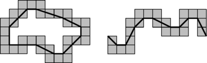
FIGURE 10.4 The length of a simple 1-curve (left) and of a simple 1-arc (right) in the 2D grid cell model [1005].
Similarly, let Mθ ⊂ ![]() be the union of all of the cells in a simple 2-arc or 2-curve in [
be the union of all of the cells in a simple 2-arc or 2-curve in [![]() , ≤]. If Mθ is a simple 2-curve, its length is the length of a minimum-length curve that is contained in Mθ and is not contractible into a single point in Mθ (see Figure 10.5, left). If Mθ is a simple 2-arc, its length is its intrinsic diameter (see Figure 10.5, right), and Mθ is a DSS iff its intrinsic diameter is defined by a straight line segment. Mθ is called planar iff the centers of all of its cells are coplanar. It can be shown that the intrinsic diameter of a nonplanar simple 2-arc is defined by a unique polygonal arc. For a given Mθ, these MLP-based length estimates are uniquely defined, but they may depend on the value of θ.
, ≤]. If Mθ is a simple 2-curve, its length is the length of a minimum-length curve that is contained in Mθ and is not contractible into a single point in Mθ (see Figure 10.5, left). If Mθ is a simple 2-arc, its length is its intrinsic diameter (see Figure 10.5, right), and Mθ is a DSS iff its intrinsic diameter is defined by a straight line segment. Mθ is called planar iff the centers of all of its cells are coplanar. It can be shown that the intrinsic diameter of a nonplanar simple 2-arc is defined by a unique polygonal arc. For a given Mθ, these MLP-based length estimates are uniquely defined, but they may depend on the value of θ.

FIGURE 10.5 The length of a simple 2-curve (left) and of a simple 2-arc (right) in the 3D grid cell model [1005].
10.1.5 Tangent-based estimation
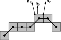
Arc length estimates can also be based on estimated tangents; see Equations 8.1 and 8.18 for the 2D and 3D cases. Figure 10.6 shows an example. An 8-path is traced along, for example, the “upper” alternating sequence of 0-cells and 1-cells of its grid cell representation. For each 1-cell, we estimate normals n1 and n2 at its endpoint 0-cells, using a DSS or MLP method to find straight line approximations to the 8-path on both sides of the 1-cell. Let n0 be the unit normal to the 1-cell, and let n = (n1 + n2)/2. We use (n, n0) = n·n0 as an approximation to ![]() Evidently, such a tangent-based length estimate depends on how the normals are estimated and combined. The normals can also be used to estimate the curvature of the path at the 1-cell.
Evidently, such a tangent-based length estimate depends on how the normals are estimated and combined. The normals can also be used to estimate the curvature of the path at the 1-cell.
In this chapter, we will study estimates of the arc lengths or curvatures of 2D digital arcs or curves, particularly with respect to their multigrid convergence; for 3D curves, see Chapter 11. Statistic properties of digital arcs and curves can also be studied; see Section 1.2.11.
10.2 Definitions of 2D Arc Length Estimators
In this section, we define the methods of 2D arc length estimation that will be evaluated in the next section.
10.2.1 Local estimators
Local estimations were historically the first ones used for arc length estimation in picture analysis. These estimators were applied to digital curves defined by digitization methods (i) or (ii) in Section 10.1.1.
Local estimators are based on shortest paths in a weighted adjacency grid of pixels. The weights are chosen to approximate Euclidean distance; see the discussion of chamfer metrics at the end of Section 3.2.3.
To make arc length estimates as accurate as possible, it has been suggested that statistic analysis be used to find weights that minimize the mean square error between the estimated and true length of a straight line segment. This leads to the definition of a best linear unbiased estimator (BLUE, for short) for straight line segments. One such estimator [281] is as follows,
where ni is the number of isothetic steps and nd the number of diagonal steps in the digital arc or curve. (The subscript “chm” refers to the chessboard metric d8.) Similar estimators have been proposed in [104] for chamfer distances (e.g., coefficients 0.95509 and 1.33693 for isothetic and diagonal steps for chamfer distances using a 3 × 3 neighborhood). Another local estimator [1115] is the cornercount estimator (coc, for short), where nc is the number of odd-even transitions in the chain code of the digital arc or curve:
Algorithms for calculating these local estimators are straightforward: trace a digital curve and locally update the estimator’s value.
10.2.2 DSS estimators
Section 9.6 reviewed algorithms for DSS recognition. These algorithms decide whether a given sequence of grid points is a DSS; some of them also segment a digital arc or curve into a sequence of maximum-length DSSs. A length estimator EDSS is then defined by the length of the resulting polygon or polygonal arc. For example, algorithm DR1995 (for 8-curves) defines the E8ss estimator, and algorithm K1990 (for 4-curves) defines the E4ss estimator. Note that the segmentation into DSSs is not uniquely defined; it depends on the method, the chosen starting point, and the direction in which the arc or curve is traced.
[283] defined a most probable original (mpo) length estimation method for DSSs that has superlinear convergence O(r−1·5); it is multigrid convergent for grid-intersection digitization and for the class of all straight line segments γ. Let n be the length of the DSS ρh,8(γ) = i(0),…, i(n−1), and let a/b be the best possible rational estimate of its slope. (Formally, b is the length of the shortest period, which is the smallest k ∈ {1,…,n} such that k = n or i(m + k) = i(m) for 0 ≤ m ≤ n – k −1. a is the height difference in one period; for example, if i(m) ∈ {0,1} for all 0 ≤ m ≤ n − 1, then a = i(0) + … + i(q − 1).) Then we have the following:
In [283], this estimator was limited to single straight line segments, but it also defines an 8-DSS-based arc length estimator 8mp: apply the 8-DSS segmentation algorithm DR1995 and sum the mpo length estimates of the 8-DSSs.
10.2.3 MLP estimators
In MLP-based length estimators, a simple 1-curve ρ is described by two isothetic polygons γ1 and γ2 that are the frontiers of sets S1 and S2 such that S2 is contained in the interior ![]() of S1 and ρ is contained in
of S1 and ρ is contained in ![]() . Here γ is defined by digitization method (iii) in Section 10.1.1, and S1 and S2 are
. Here γ is defined by digitization method (iii) in Section 10.1.1, and S1 and S2 are ![]() and
and ![]() , with the constraint that γ1 and γ2 are at Hausdorff distance 1 with respect to L∞. We find an MLP that is contained in B and circumscribes γ2; the Emlp length estimate is then the length of this (uniquely defined) MLP.
, with the constraint that γ1 and γ2 are at Hausdorff distance 1 with respect to L∞. We find an MLP that is contained in B and circumscribes γ2; the Emlp length estimate is then the length of this (uniquely defined) MLP.
We will describe two MLP-based length estimators. The standard MLP estimator Emlp defines B to be the difference set between the outer and inner Jordan digitizations of S. The approximating-sausage estimator Eaps also involves a parameterδ (0 <δ ≤ 0.5/h).
10.2.4 MLPs of simple 1-curves
We assume that γ1 and γ2 are traced in the positive orientation (i.e., counterclockwise in a righthand coordinate system). A vertex vi on γ1 or γ2 is called a convex vertex if the frontier makes a positive turn at vi (i.e., D(vi−1, vi, vi + 1) > 0 [see Equation 8.14]). Similarly, vi is called a concave vertex if the frontier makes a negative turn (D(vi−1, vi, vi + 1) < 0) and a collinear vertex if D(vi−1, vi, vi+1) = 0.
Our algorithm traces γ1 (or γ2), detects convex and concave vertices, puts their coordinates into a list L, and marks them as convex or concave. For simplicity, assume that the coordinates are integers. The coordinates of two successive vertices with indices i and i + 1 satisfy |xi + 1 – xi| + |yi + 1 –yi| = 1.
It is easy to show that only convex vertices of the “inner ” curve γ2 and only concave vertices of the “outer ” curve γ1 can be vertices of the MLP. There exists a mapping from the set of all concave vertices of γ2 onto the set of all concave vertices of γ1 such that each concave vertex of γ1 corresponds to at least one concave vertex of γ2. See Figure 10.7 for an example. The numbers denote successive vertices in the list L; 1 is a start vertex (i.e., an already known MLP vertex); 3 and 5 are successive convex vertices on γ2; 2, 4, and 6 are successive concave vertices on γ1. Vertex 7 is not between the negative (black line) and positive (white line) sides of sector (6,1,5); therefore 5 is the next MLP vertex and is a new start vertex.
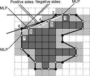
FIGURE 10.7 Finding the next MLP vertex [555].
The algorithm starts by putting all of the vertices of γ2 into L. We then replace each concave vertex of γ2 in L with its corresponding concave vertex of γ1 by modifying its coordinates by ±1, where the sign depends on the orientations of the incident edges. L now contains all of the vertices that will form the MLP. Note that the vertices in L are still in the original vertex order on γ2.
Suppose we already know that vertex vi of L is an MLP vertex. Then vj (j > i) can be an MLP vertex only if all convex vertices ![]() such that i < k < j lie on the positive side of (vi, vj) or are collinear with it (i.e., D(vi,
such that i < k < j lie on the positive side of (vi, vj) or are collinear with it (i.e., D(vi,![]() , vj) ≥ 0). Similarly, all concave vertices
, vj) ≥ 0). Similarly, all concave vertices ![]() such that i < l < j must lie on the negative side of (vi, vj) or be collinear with it. (Otherwise (vi, vj) would cross either γ1 or γ2, which is not allowed to happen.) Suppose a convex vertex v + and a concave vertex v− both satisfy these conditions. When we consider a vertex v as a candidate MLP vertex, the following situations can occur:
such that i < l < j must lie on the negative side of (vi, vj) or be collinear with it. (Otherwise (vi, vj) would cross either γ1 or γ2, which is not allowed to happen.) Suppose a convex vertex v + and a concave vertex v− both satisfy these conditions. When we consider a vertex v as a candidate MLP vertex, the following situations can occur:
1. v lies on the positive side of (vi, v +) (i.e., D(vi, v +, v) ≥ 0);
2. v lies on the negative side of (vi, v +) or is collinear with it and also lies on the positive side of (vi, v−) or is collinear with it; or
In case (1), v + becomes the next MLP vertex. In case (2), v becomes a candidate for the MLP and must replace either v + or v− depending on the sign of v. In case (3), v− becomes the next MLP vertex. This is also correct in the trivial case where v +, v−,or both coincide with vi. Thus we can start with a vertex v1 that is known to be an MLP vertex (e.g., the uppermost-leftmost vertex of γ2); set v + and v− equal to v1; and then test all subsequent vertices as just described. Whenever the next MLP vertex is detected, it becomes a new start vertex.
The algorithm is given in Algorithm 10.1; it also provides a length estimate L.
If we are given a simply connected 4-component in the grid point model, the 4-path through all of the 8-border points of S defines the inner frontier γ2. We can expand γ2 into an outer frontier γ1 at Hausdorff distance 1 from γ2 (with respect to L∞) and use γ1 and γ2 as inputs for the MLP algorithm. Figure 10.8 shows that the algorithm can handle “narrow concavities.” The resulting MLP intersects all of the invalid edges of S.

FIGURE 10.8 Successive steps of the MLP algorithm. In this example, γ1 and γ2 cross one another at A, and different segments of γ1 coincide at the three Bs [555].
Figure 10.8 also illustrates how the algorithm proceeds. The top left shows an example of the set between γ1 and γ2. The top right shows the original sequence
of 8-border points as a dark curve (γ2); the bottom left shows the curve that connects all convex vertices on γ2 and concave vertices on γ1 in the order tested in the algorithm; and the bottom right shows the resulting MLP. The algorithm has linear time complexity.
10.2.5 The approximating sausage approach
Let the h-frontier of S be represented by Π = (v0, v1…, vn−1) where the vertices are in clockwise order and the interior of S lies to the right. We define the forward shift f (vi) of vi as the point on the edge (vi, vi + 1) at distanceδ from vi, and the backward shift b(vi) of vi as the point on the edge (vi−1, vi) at distance δ from vi.
To generate the approximating sausage “around” Π, for each edge (vi, vi + 1), we define the line segment (vi, f(vi + 1)) that joins vi to the forward shift of vi + 1; this is referred to as the forward approximating segment and is denoted by Lf (vi). The backward approximating segment (vi, b(vi−1)) is defined similarly and denoted by Lb(vi). We now have three sets of edges: the original edges of the h-frontier and the forward and backward approximating segments. Using these edges, we define a connected region ![]() that is homeomorphic to an annulus as follows:
that is homeomorphic to an annulus as follows:
Given a polygonal circuit Π that describes an h-frontier in clockwise orientation, by reversing Π, we obtain a polygonal circuit Π−1 in counterclockwise orientation. In the initialization step of our approximation procedure, we consider Π and Π−1 as the external and internal bounding polygons of a polygon ΠB that is homeomorphic to the annulus. This initial polygon ΠB has area 0, and its points coincide with those of ϑh(S).
We now “move” the external polygon Π “away” from Gh(S) and the internal polygon Π−1 “into” Gh(S), as described below. (The Hausdorff distance between Π and Π−1 is nonzero when the sets are not identical.) This process expands ΠB step by step into a final polygon that containsϑh(S), and such that the Hausdorff distance between Π and Π−1 is always less than or equal to 1/h. For this purpose, we add forward and backward approximating segments to Π and Π−1 to increase the area of ΠB.
In the “moving” process, for any forward or backward approximating segment Lf (vi), or Lb(vi), we first remove the part lying in the interior of the current polygon ΠB and update ΠB by adding the remaining part of the segment as a new frontier edge. The orientation of this edge is chosen so that the interior of ΠB lies to the right of it. The resulting polygon ![]() is referred to as the approximating sausage of the h-frontier and is denoted by
is referred to as the approximating sausage of the h-frontier and is denoted by ![]() (see Figure 10.9, left, for δ = 1/2). Note that the width of the approximating sausage depends on δ. An aps approximation of the frontier of S is a shortest closed curve
(see Figure 10.9, left, for δ = 1/2). Note that the width of the approximating sausage depends on δ. An aps approximation of the frontier of S is a shortest closed curve ![]() that lies entirely in the interior of
that lies entirely in the interior of ![]() and encircles the internal frontier of
and encircles the internal frontier of ![]() (see Figure 10.9, right). It follows that
(see Figure 10.9, right). It follows that ![]() is uniquely defined and is a polygonal curve defined by finitely many straight line segments. Note that
is uniquely defined and is a polygonal curve defined by finitely many straight line segments. Note that ![]() depends on the choice of δ; we have used δ = 0.5/h in our experiments.
depends on the choice of δ; we have used δ = 0.5/h in our experiments.

FIGURE 10.9 Left: construction of the approximating sausage. Right: resulting aps curve [50].
10.2.6 Tangent-based estimators
We can use a tangent vector integration process to estimate the length of a curve; see Equation 8.1. Let ![]() be the length of the tangent vector associated with γ(t). Then the following can be approximated by using discrete estimates of the products
be the length of the tangent vector associated with γ(t). Then the following can be approximated by using discrete estimates of the products ![]() dt:
dt:
To estimate the normals n1 and n2 (see Figures 10.6 and 10.10), we regard the 0-cell as the center point p of a maximum-length DSS of the 8-curve that is obtained by tracing one frontier of the digitized (in the grid cell model) curve γ. A centered maximum-length DSS always has even length. The estimates can also be based on 4-DSSs that approximate the 4-curve of the chosen frontier. Figure 10.10 shows a DSS approximation on the left and a 4-DSS approximation on the right.

FIGURE 10.10 Left column: DSS centered at p. Right column: 4-DSS centered at p. Upper row: estimation of n1; both estimated tangential lines, and hence both estimated normals, are identical. Lower row: estimation of n2; different estimated tangential lines result in different estimated normals, depending onhowthe estimator is defined.
The DSS (or 4-DSS) approximates the tangent line to γ, and the normal is perpendicular to this line. This method can make use of any DSS definition and recognition algorithm. Straightforward application of a linear online DSS recognition algorithm starting at p and proceeding alternatingly in both directions along the curve leads to an ![]() solution, where n is the number of pixels on the curve.
solution, where n is the number of pixels on the curve.
An optimization method proposed in [323] allows us to compute all of the discrete tangents in linear time by using the discrete tangent computed at each vertex to initialize the discrete tangent at the next vertex; on average, this requires only a constant number of changes. We will use DSS approximation of the outer frontiers of simple 0-curves. The discrete version of Equation 10.4 is as follows, where S is the set of all pixels in digh(γ):
For each 1-cell c in the alternating sequence of 0-cells and 1-cells along the chosen frontier, we calculate n(c) and n0(c).
10.3 Evaluation of 2D Arc Length Estimators
This section presents both experimental and theoretic comparisons of the 2D arc length estimators that were described in Section 10.2.
10.3.1 Online and offline algorithms and time complexity
The notions of online, offline, and linear time apply to estimators of all four classes; we describe them here for DSS estimators (see Section 9.6). An offline DSS algorithm takes an entire arc or curve (defined by a finite word u ∈ A*) as input and decides whether it is a DSS. An online DSS algorithm reads successive chain codes i(0), i(1),…; for each n, it decides whether i(0),i(1),…, i(n) is a DSS; if not, it initializes a new DSS with i(n − 1)i(n). After a maximum-length DSS has been found, its length estimate (usually the Euclidean distance between its end vertices) is added to the length estimate of the arc or curve. An offline algorithm is linear iff it runs in ![]() time (i.e., it performs at most
time (i.e., it performs at most ![]() basic computation steps for any input word u ∈ A*). An online algorithm is linear iff it performs on the average a constant number of operations for each chain code symbol.
basic computation steps for any input word u ∈ A*). An online algorithm is linear iff it performs on the average a constant number of operations for each chain code symbol.
10.3.2 Multigrid convergence theorems
We apply the general definition of multigrid convergence (Definition 2.10) to the problem of estimating the length L(γ) of an arc or curve γ. Assume that the estimate E is defined for all curves γ in a given class (e.g., the class of all simple curves in the Euclidean plane) and for all digitizations digh(γ) where h > 0. E is multigrid convergent to L with respect to digitization model digh iff E(digh(γ)) converges to L(γ) as h → ∞ for any curve γ in the class of interest. More formally, we have the following:
where limh→∞ κ(h) = 0; the speed of convergence is ![]() .
.
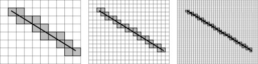
In general, we expect that an increase in grid resolution will result in an increase in accuracy. Suppose the digitization of a straight line segment consists of all cells that have nonempty intersections with the segment (i.e., we use outer Jordan digitization; see Figure 10.11). If the grid resolution is h > 0, the Hausdorff distance between the segment and the frontier of its outer Jordan digitization is ![]() . Hence the frontier converges to the segment with respect to the Hausdorff metric generated by the Euclidean metric. However, the perimeter of the union of the cells remains constant as h increases; this shows that this perimeter cannot be used for length estimation.
. Hence the frontier converges to the segment with respect to the Hausdorff metric generated by the Euclidean metric. However, the perimeter of the union of the cells remains constant as h increases; this shows that this perimeter cannot be used for length estimation.
The local estimators chm and coc of the lengths of digitized arcs or curves (see Section 10.3) are not multigrid convergent. No proof has yet been published that local estimators cannot achieve multigrid convergence for “sufficiently complex” input data (e.g., not just for isothetic rectangles).2 Given an algorithm for constructing a DSS approximation of the h-frontier ![]() of a simply connected digital set Gh(S), we define εDSS/h as the maximum Hausdorff distance between
of a simply connected digital set Gh(S), we define εDSS/h as the maximum Hausdorff distance between ![]() and γh:
and γh:
Theorem 10.1
Let S be a convex h-compact polygonal set in ![]() . Then there exists a grid resolution h0 such that, for all h ≥ h0, any DSS approximation of the h-frontier
. Then there exists a grid resolution h0 such that, for all h ≥ h0, any DSS approximation of the h-frontier ![]() is a connected polygon with perimeter Ph that satisfies the following inequality:
is a connected polygon with perimeter Ph that satisfies the following inequality:
(This theorem is from [560]; for a proof, see Section 10.3.3.) The value of h0 depends on the given set. If εDSS (h) = 1/h, it follows from Equation 10.8 that the upper error bound for DSS approximations is as follows3:
In [883], a DSS is assumed to be a finite 8-path. When we use cell complexes, it is appropriate to consider a finite 4-path to be a DSS iff its main diagonal width is less than ![]() ; see [20, 597, 848].
; see [20, 597, 848].
Both of the MLP-based arc length estimators described in Section 10.2 (mlp and aps) are known to be multigrid convergent for convex Jordan curves γ.
Theorem 10.2
Let S be a bounded h-compact convex polygonal set. Then there exists a grid resolution h0 such that, for all h ≥ h0, any aps approximation of the h-frontier ![]() (0 <δ ≤ 0·5/h) is a connected polygon, for example, with perimeter Ph and the following:
(0 <δ ≤ 0·5/h) is a connected polygon, for example, with perimeter Ph and the following:
There are several convergence theorems for MLP approximations in [1005]. The perimeter of such an approximation is a convergent estimator of the perimeter of a bounded convex smooth or polygonal set in the Euclidean plane. The following theorem is basically from [1005]; it specifies the asymptotic constant for mlp perimeter estimates.
Theorem 10.3
Let γ be a convex planar curve that is contained in a simple 1-curve ρ in [![]() 2, ≤] for grid resolution h ≥ 1. Then the MLP approximation of ρ is a connected polygonal curve of length Ph that satisfies the following:
2, ≤] for grid resolution h ≥ 1. Then the MLP approximation of ρ is a connected polygonal curve of length Ph that satisfies the following:
From Theorems 10.1, 10.2, and 10.3, we see that the DSS upper error bound 4·5/h is smaller than the aps upper bound 5·844/h, which is in turn smaller than the mlp upper bound 8/h. However, this does not imply anything about the relative size of these errors. The determination of optimum error bounds remains an open problem.
The speed of convergence and the maximum error bound for these estimates have not yet been determined.
10.3.3 Proof of Theorem 10.1
To prove Theorem 10.1, we use two lemmas from integral geometry [958].
We recall that an ε-sausage of a curve γ (as originally discussed by H. Minkowski [732]; see Figure 7.2) is the set of all points ρ such that de({p}, γ) ≤ε.
We now prove Theorem 10.1. We assume that S is h-compact for h ≥ h0, so Gh(S) is connected, and the DSS approximation of ![]() is a single (connected) polygonal curve. We will prove that there exists a constant h1 ≥ 1 such that the following is true for all h ≥ h1:
is a single (connected) polygonal curve. We will prove that there exists a constant h1 ≥ 1 such that the following is true for all h ≥ h1:
Suppose this Hausdorff distance was greater than ![]() . Then there would exist either (A) at least one point p on
. Then there would exist either (A) at least one point p on ![]() with a minimum Euclidean distance to
with a minimum Euclidean distance to ![]() that is greater than
that is greater than ![]() or (B) at least one point q on ϑS with a minimum Euclidean distance to
or (B) at least one point q on ϑS with a minimum Euclidean distance to ![]() that is greater than
that is greater than ![]() .
.
In case (A), the circle with centerρ and radius ![]() would not contain any point of ϑS; hence this circle would be either (A1) disjoint from S or (A2) completely inside of S. Let p be on the frontier of a grid square with midpoint
would not contain any point of ϑS; hence this circle would be either (A1) disjoint from S or (A2) completely inside of S. Let p be on the frontier of a grid square with midpoint ![]() . The grid point
. The grid point ![]() is inside the circle. In case (A1), it follows that
is inside the circle. In case (A1), it follows that ![]() cannot be in S (i.e.,
cannot be in S (i.e., ![]() is not in Gh(S)). It follows that p cannot be on ϑh(S), which contradicts our assumption. In case (A2), p is on an h-edge incident with two h-squares with midpoints that are both in the circle and thus in S; hence, in this case, too, p cannot be on ϑh (S). Thus case (A) is impossible.
is not in Gh(S)). It follows that p cannot be on ϑh(S), which contradicts our assumption. In case (A2), p is on an h-edge incident with two h-squares with midpoints that are both in the circle and thus in S; hence, in this case, too, p cannot be on ϑh (S). Thus case (A) is impossible.
In case (B), because S is h-compact for h ≥ h0, the distance between q and the nearest grid point can become arbitrarily small as h → ∞, while Gh(S) still remains connected. Thus, in case (B), we must increase h so that h ≥ h1 ≥ h0 for some h1, which represents the situation in which the minimum Euclidean distance from q ∈ ![]() to
to ![]() is less than or equal to
is less than or equal to ![]() . Only a finite number of vertices on the frontier of S can require such increases in h0. This concludes the proof of Equation 10.12.
. Only a finite number of vertices on the frontier of S can require such increases in h0. This concludes the proof of Equation 10.12.
Equations 10.12 and 10.7 and the triangle inequality for Hausdorff distance imply the following:
Let ![]() . Then the perimeter of S and the length of γh differ by at most 2πε. To show this, let γh be the frontier of a convex (polygonal) set C so that the following is true:
. Then the perimeter of S and the length of γh differ by at most 2πε. To show this, let γh be the frontier of a convex (polygonal) set C so that the following is true:
We will show that the following is true, which will complete the proof of the theorem:
The frontier ![]() lies in the ε-sausage of the frontier
lies in the ε-sausage of the frontier ![]() . Let
. Let ![]() be the outer frontier of the ε-sausage of
be the outer frontier of the ε-sausage of ![]() . By Lemma 10.1, we have the following:
. By Lemma 10.1, we have the following:
By Lemma 10.2, we have the following:
![]() lies in the ε-sausage of
lies in the ε-sausage of ![]() , because Hausdorff distance is symmetric. Let
, because Hausdorff distance is symmetric. Let ![]() be the outer frontier of the ε-sausage of
be the outer frontier of the ε-sausage of ![]() . By Lemma 10.1, we have the following:
. By Lemma 10.1, we have the following:
By Lemma 10.2, we have the following:
From Equations 10.15 and 10.16, we have the following
which proves Equation 10.14 and thus the theorem.
10.3.4 Experimental evaluation
Comparative evaluations of length estimators should investigate their accuracy and stability both on convex and nonconvex curves. In the experiments reported in [206], we used the test curves shown in Figure 10.12 digitized on grids of sizes between 30 × 30 and 1000 × 1000 using any of the three digitization methods in Section 10.1.1.

FIGURE 10.12 Test curves [555].
Two performance measures were used: (i) the relative error (in percent) between the estimated and true curve length; and (ii) for the DSS and MLP methods, a tradeoff measure defined as the product of the relative error and the number of generated segments (the efficiency of convergence).
In the plots in Figure 10.13, convergence is evident for all of the estimators. However, for estimators chm and coc, the convergence is to a false value! The errors are calculated for each curve, combined into a mean error for each grid size, and then the plots are generated by taking sliding means over 30 grid sizes. We show both linear and logarithmic plots of the errors. 8mp slightly overestimates the length as compared with 8ss.

FIGURE 10.13 Multigrid convergence of length estimators: plots of sliding means of the relative errors (above); logarithmic plots (below) [206].
The tradeoff measure is plotted in Figure 10.14 for the DSS and MLP estimators. Here, too, the errors are calculated for each curve and combined into a mean error for a given grid size, and the plots are generated by taking sliding means over 30 grid sizes.

FIGURE 10.14 Trade off plots for the DSS and MLP estimators [206].
As an additional test, a square of fixed size was rotated in a grid of resolution 128. Figure 10.15 shows its estimated perimeter as a function of rotation angle. Except for chm and coc, the estimates are relatively orientation-independent.
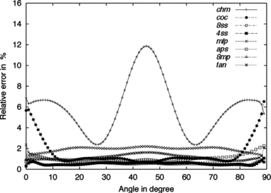
FIGURE 10.15 Relative errors for a rotating square [206].
Figure 10.16 shows the runtimes of the DSS and MLP estimators as compared with local estimators. Obviously, the local estimators are fastest. MLP as implemented in [555] (as described in Section 10.2.3) is the fastest global estimator, but 4ss and 8ss come close to it. The aps estimator has not yet been optimized; faster implementations may be possible. Theoretically, the tan estimator has a linear asymptotic runtime implementation [323], but the estimator that was tested had quadratic runtime; optimization is needed here, too.

FIGURE 10.16 Runtimes of the DSS- and MLP-based estimators on an Ultra 10 Sparc workstation [206].
These experiments show that the local estimators are not multigrid convergent even for our simple test data set. For the five global estimators, we obtained experimental confirmations of known theoretic convergence results.
Interestingly, the runtimes of the polygonal DSS and MLP estimators were only slightly greater than those of the local estimators; hence the use of local estimators is not justified by a runtime argument. The choice of a global estimator may depend on the available software. Studies involving more extensive test data might be useful in the selection of the most efficient estimator for a given application.
All of the tested estimators have linear online complexity. Of all of the possible MOP extensions of the DSS and MLP estimators we have reported only on 8mp. Our theoretic studies answered (in most cases) the following questions:
multigrid convergence: Is the estimator multigrid convergent at least for convex curves? (If so, we are also interested in its convergence speed.)
discrete: Does the core of the estimation algorithm deal only with integers?
unique: Is the result independent of initialization (starting point, tracing orientation, and so forth)?
3D extension: Can the estimator be extended to digital curves in 3D space?
Table 10.1 provides a summary of the answers to these questions. Convergence speed is known to be linear for 8ss, 4ss, mlp and aps; see Theorems 10.1,10.2,10.3, and 10.4.

10.4 The Curvature of a Planar Digital Curve
In this section, we discuss methods of estimating the curvature of a planar curve and detecting “corners” (high-curvature pixels) on such curves. Let ρ = (pv…, pm) be an α-curve (usually an 8-curve) in ![]() . Let pi = (xi, yi), where i = 1,…, m, and let 1 ≤ k ≤ m. For each pixel pi onρ, we define a forward vector fi,k = pi – pi + k and a backward vector bi,k = pi – pi–k, where the indices are modulo m. Let
. Let pi = (xi, yi), where i = 1,…, m, and let 1 ≤ k ≤ m. For each pixel pi onρ, we define a forward vector fi,k = pi – pi + k and a backward vector bi,k = pi – pi–k, where the indices are modulo m. Let ![]() and
and ![]() .
.
10.4.1 Corner detectors
Curvature analysis is often oriented toward detecting high-curvature pixels (“corners”). We first review two early methods that detect such pixels without calculating curvature estimates.
Algorithm RJ1973
This algorithm [910] detects a corner at pi based on analysis of the cosines ci,k of the angles between the forward vector fi,k and the backward vector bi,k; ci,k is called the k-cosine angle measure. Let 0 < a < 1 (e.g., a = 0.05) and  . We start at k = k0 and decrement k as long as ci, k increases. Suppose this occurs at k = ki so that ci ki ≥ ci,k−1. In a subsequence ofρ of length ki centered at pi
a corner is detected at pi iff ci,ki > ci,kj for all j ≠ i such that |i – j| ≤ ki/2 (modulo m).
Note that the algorithm depends on only one parameter a. Because it does not use a constant initial value k0, it is adaptive to the length of the 8-curve and is therefore global.
Algorithm RW1975
This algorithm [924] uses averaged cosine values given here:

Otherwise, it follows algorithm RJ1973.
The k-cosine angle measure is an example of a significance measure defined in a sliding interval of width 2k0 + 1 and evaluated in a reduced interval of width k0 + 1.
The parameter k0 depends on the number m of points on the given digital curve. The sliding interval defines a region of support (ROS) for a detected corner, which is normally considered to be at the center of its ROS. Evaluation of the measure is limited to a subset of the ROS. In the aforementioned examples, the size [am] of the ROS is uniformly determined (i.e., it is the same at every point of the curve).
[703] reviews more than 100 corner detection and curvature estimation algorithms for 2D digital curves. Curvature estimators (C1) will be reviewed in the next subsection. Other approaches are based on the following:
(C2) Estimation of curve properties in a uniformly determined ROS defined by input parameters. Examples of relevant properties are (C2.1) angles between forward and backward vectors (see above); (C2.2) approximation errors (e.g., defined by distances between arcs and chords [see Figure 10.17]); and (C2.3) directional changes between forward and backward ROSs.
(C3) Estimation of curve properties in an individual determined ROS.
In the following paragraphs, we give a few examples of such approaches.
[251] uses approach (C2.1) at various scales to polygonally approximate the curve at different levels of detail. [257] defines multiscale curvature based on minima and maxima of the k-cosine at different scales, where k varies with the scale. In [194], corners are locations at which a triangle of specified size and angle can be inscribed in the curve.
Two of the corner detectors proposed in [932] are based on approach (C2.2), specifically on distances between arcs and chords (see Figure 10.17). In [327], points of the curve are classified into the categories “on smooth interval,” “on noisy interval,” and “corner” by analyzing deviations of arcs of the curve from their chords. A more efficient implementation of this method was presented in [815]. Arc-chord distance is combined with Gaussian scale-space techniques in [407].

FIGURE 10.17 The arc-chord distance measure is defined by the distance d between a point p on the curve and a symmetric chord defined by a parameter k.
As an example of approach (C2.3), [295] defines a curvature chain ci = mod8 (si – si−1 + 11) − 3 where the sis are chain codes. This curvature chain is “smoothed” by convolution with a filter. [46] uses comparisons of forward and backward chain code histograms based on a correlation coefficient measure. Chain code histograms on a sliding arc are used in [47].
Other approaches based on curve properties include analysis of the chord lengths between pairs of points k steps apart along the curve [603] or of the number of DSSs centered at a point of the curve [586]. Corners can also be defined by local maxima of a measure of local symmetry [782]. [1065] describes a corner detection method based on eigenvalues of covariance matrices of neighborhoods of curve points.
As an example of approach (C3), studies of the visual perception of shapes [618] motivated [879] to assign individually sized neighborhoods to border points of convex regions to detect “dominant points.” [837] gives an algorithm for the calculation of backward and forward vectors and also allows asymmetric ROSs at a point. The backward and forward vectors point to pi–k and pi + i, respectively, where k and l are determined by studying the angular changes that take place when moving away from pi along the curve. A (k, l)-cosine measure is used to detect corners; see [838] for further studies along these lines. For a combination of multiscale and individually sized ROSs, see [770].
Finally, we mention two examples of other approaches (C4). In [455], chain codes are transformed into differential chain codes ci = si – si−1. The maximum lengths of nonzero sequences in the differential code – and sums of consecutive nonzero differential codes (starting with pair sums and generalizing to group sums) – are used to detect “critical points.” See [32] for other applications of differential codes. [421] derives a hierarchical, polygonal approximation to a curve by detecting candidate “dominant points” and then iteratively removing “least significant points” until a stable polygonal approximation is reached.
10.4.2 Curvature estimators
Curvature can be estimated from (C1.1) the change in the slope angle of the tangent line (e.g., relative to the x-axis); (C1.2) derivatives along the curve; or (C1.3) the radius of the osculating circle (circle of curvature); see Definition 8.1, Equation 8.9, and Equation 8.11, respectively.
Algorithm FD1977
This algorithm [346] (in category (C1.1)) estimates changes in the slope angles θi of the tangent lines at points pi. Let the following be the angle estimate based solely on backward vectors of “length” k:

Let the following be the centered difference,
which is “accumulated” by the following using Δ = tan−1(1/(k −1)):
Let the following also be true:
These are the maximum lengths of the arcs preceding pi and following pi + k in which the differences δj,k remain close to zero (in an interval [–Δ, + Δ]) and which define the “legs” of a corner.
A corner is detected at pi iff Ei,k > T and the previous corner is at a distance of at least k from pi on ρ.
Note that this procedure depends on a parameter k (e.g., k = [am] as in algorithm RJ1973) and on a threshold T. Because t in the definition of t1 and t2 can be arbitrarily large, this is a global method.
Algorithm BT1987
This algorithm [84] modifies algorithm FD1977 as follows: t1 and t2 are upper-bounded by ![]() (0 < b < 1), and the curvature estimates Ei,k are calculated and averaged over a range of values of k (kL ≤ k ≤ kU):
(0 < b < 1), and the curvature estimates Ei,k are calculated and averaged over a range of values of k (kL ≤ k ≤ kU):
This method involves four parameters: kL, kU, b, and the threshold T. Because the upper bound is [bm], it is a global method.
Algorithm HK2003
This algorithm [434], which is also in category (C1.1), estimates changes in the slope angles of tangents. It calculates a maximum-length 8-DSS pi-bpi of the following Euclidean length
that goes “backward ” from pi onρ and a maximum-length 8-DSS pipi + f of the following length

that goes “forward” from pi on ρ. It then calculates the following angles,

the mean θi = θb/2 +θf/2, and the angular differences δ1 = |θf −θi | and δ2 = |θb −θi|. Finally, the curvature estimate at pi is as follows:
Algorithm M2003
[736] is an early example of an algorithm in category (C1.2). More recently, [703] assumes that the given 8-curve 〈p1,…, pm〉, where pj = (xj, yj) for 1 ≤ j ≤ m,is sampled along a parameterized curve γ(t) = (x(t),y(t)) where t ∈ [0,m]. At point pi, we assume that γ(0) = γ(m) = pi and γ(j)= pi+j for 1 ≤ j ≤ m −1. Functions x(t) and y(t) are locally interpolated at pi by the following second-order polynomials,
and curvature is calculated using Equation 8.9. We have x(0) = xi, x(1) = xi-k, and x(2) = xi + k with integer parameter k ≥ 1; this is analogous for γ(t). The curvature at pi is then defined by the following:
Algorithm CMT2001
This algorithm [208], which is in category (C1.3), involves approximation of the radius of the osculating circle. At each point pi, we calculate a maximum-length DSS centered at pi. This DSS is used as an approximate segment of the tangent at pi, and its length li corresponds to the radius of the osculating circle. The algorithm calculates an inner radius Ii =[li − 1/2)2 − 1/4] and an outer radius Oi = [(l + 1/2)2 − 1/4] and returns 2/(Ii + Oi) as an estimate of the radius of curvature at pi.
10.4.3 Experimental evaluation
[661] contains an experimental comparison of several curvature estimation methods (see Sections 10.4.1 and 10.4.2) that were published before 1990 as well as some other local methods (see the references in Section 10.6). The results obtained from algorithm BT1987 were described as being “in best correspondence to human perception.”
We illustrate comparative evaluations for only two algorithms, CMT2001 and HK2003. The curvature of a circle of radius R is κ = 1/R. Figures 10.18 and 10.19 show the error ![]() averaged over all pixels on 8-curves that are the borders of Gauss digitizations of disks x2 + y2 = r2 or x2 + y2 = r2 + r (r = 100,…, 1000). The plots are sliding means, which eliminate “digitization noise” by symmetrically averaging 19 values before and 19 values after the current value r.
averaged over all pixels on 8-curves that are the borders of Gauss digitizations of disks x2 + y2 = r2 or x2 + y2 = r2 + r (r = 100,…, 1000). The plots are sliding means, which eliminate “digitization noise” by symmetrically averaging 19 values before and 19 values after the current value r.

FIGURE 10.18 Left: sliding means of errors in the interval [0,…, 0.01] for algorithms CMT2001 (upper curve) and HK2003 (lower curve) for the digitized disk x2 + y2 = r2 + r. Right: sliding means of errors in the interval [0…0.02] for x2 + y2 = r2 and x2 + y2 = r2 + r; the upper pair of curves are for CMT2001 and the lower pair for HK2003. In both cases, the (larger!) disk x2 + y2 = r2 + r produces smaller errors.

FIGURE 10.19 Sliding means of errors for algorithm HK2003 (lower curve) for the disk x2 + y2 = r2 digitized at grid resolutions h = 100,…, 1000, as compared with local restrictions of the algorithm in which the length of the approximating line segments is limited to 5 (upper curve) or 7 pixels. The curves intersect between r = 100 and r = 101 and between r = 203 and r = 204.
Figure 10.18 shows total errors for algorithms CMT2001 and HK2003, on the left for the digitized disk x2 + y2 = r2 + r and on the right also for the disk x2 + y2 = r2. In the latter case, the digital disk has small “peaks” on its border due to the fact that its radius is an integer. These “unsmooth” situations slightly increase the error for both algorithms.
Figure 10.19 shows how the errors behave if the unlimited-length DSS approximation in HK2003 is replaced by backward bi,k and forward vectors fi,k of constant length (5 and 7 in the figure). The errors are smaller than for the global method up to about r = 100 for k = 5 and up to about r = 200 for k = 7.
[703] contains an extensive experimental comparison of corner detectors and curvature estimation methods; it demonstrates good performance of algorithm M2003 as compared with 28 other methods. We illustrate the experimental comparison in [703] by giving results obtained by five methods on two 8-curves (4-borders of 4-regions); Figure 10.20 shows these 8-curves.
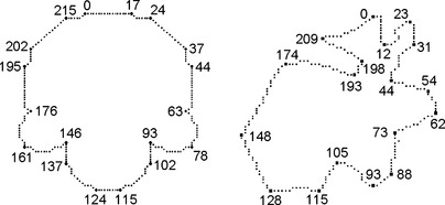
FIGURE 10.20 A symmetric 8-curve (left) and an asymmetric 8-curve (right) that were used in comparisons of corner detectors (using only the grid resolution shown in the figure).
Figure 10.21 shows corner or curvature values for the symmetric curve (which is of length 222) calculated by methods RJ1973 (with a = 0.1), FD1977 (with k = 9), BT1987 (with kL = 9, kU = 14, and b = 0.1), M2003 (with k = 10), and HK2003.

FIGURE 10.21 Corner or curvature values measured by five methods. The parameters used are specified in the figure. The x-coordinate gives border point numbers as shown in Figure 10.20 for the symmetric curve.
RJ1973 produces a “plateau” between border points 115 and 124. The original algorithm would label all of these points as being corners. In the resulting segmentation, which is shown in Figure 10.22 on the upper left, only the midpoint of this “plateau” is taken as a corner.

FD1977 reproduces the curve’s symmetry in the calculated values Ei,k. The original algorithm maps these into asymmetric corner positions; see the segmentation shown in Figure 10.22, which uses k = 9. The following modification would produce perfectly symmetric corners: select pi as a corner iff Ei,k > Ej,k for all j such that |i – j| ≤ k.
A maximum of 14 corners was used for BT1987. No corners were detected by FD1977 at any of pixels 63 through 93 or 146 through 176.
Threshold 0.08 was used for corner detection in M2003. This algorithm also detects subsequences of corners that are “nearly collinear”; see the three corners on the left and on the right in Figure 10.22. Elimination of corners that are nearly collinear with the preceding and following corners would eliminate this type of redundancy.
Method HK2003 does not require any specification of parameters, but it depends on the orientation in which the border is traversed. The curvature values are not symmetric because a maximum-length DSS from pi to pj is not necessarily a maximum-length DSS from pj to pi. At each pi, a “backward interval” and a “forward interval” are defined by backward and forward DSSs. A corner is detected iff the curvature at pi is at least equal to the curvatures at every pj in pis backward and forward intervals.
Figure 10.24 shows corner or curvature values for the asymmetric curve in Figure 10.20 (which has length 223) calculated by the same five methods. The resulting segmentations are shown in Figure 10.23.

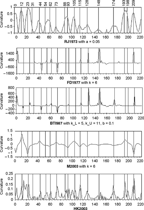
FIGURE 10.24 Corner or curvature values measured by five methods. The parameters used are specified in the figure. The x-coordinate gives border point numbers as shown in Figure 10.20 for the asymmetric curve.
10.5 Exercises
1. The Archimedes-Hui constant of a length estimation algorithm is the minimum grid resolution h0 such that the algorithm initially estimates π within the error interval defined by Equation 1.6 when a circular region centered at the origin is digitized in a grid with edge length 1/h. Note that the estimates “oscillate,” so later estimates may be outside of this interval. Using a sliding mean is critical because the behavior of the errors is uncertain. Can you give a “better” definition of such a constant? Calculate the constants (using the above definition or an improved definition) for DSS and MLP length estimation methods.
2. Consider the inner and outer Jordan digitizations of a bounded connected planar set S and the MLP contained in the difference set of the two digitizations and circumscribing the inner digitization. Identify cases in which the grid-intersection digitizations of this MLP and of the frontier of S are (are not) the same.
3. In cases A and B in Figure 10.8, two border vertices are at distance 1 or 2 in the grid but at distance greater than 2 on the border 4-curve. Prove that the Algorithm 10.1 produces a grid polygon that circumscribes the inner polygon, even in cases A and B.
4. If two grid cells that share an edge e in a 2D multivalued picture P have values u and v, we say that e has strength |u – v|. The sum of the strengths of all of the grid edges in P is called the total frontier strength of P. Prove that, if P is binary, its total frontier strength is equal to the sum of the lengths (in grid edge units) of all of the frontier of P along which 0s meet 1s.
5. Implement algorithm M2003 and at least one other curvature estimation algorithm of your choice, and evaluate their performance as was done in Section 10.4.3.
6. Let ρ be a 4-path with pixels p1,…, pn that are all distinct. At each pixel pi (1 < i < n), the path is either straight or makes a right or left turn, depending on whether the determinant D(pi−1, pi, pi + 1) is zero, positive, or negative. In these cases, we say that the turn of ρ at pi is 0, π/2, or −π/2, respectively;θi is the turn ofρ at pi. If p1 is a 4-neighbor of pn (so that the path defines a closed curve), we can also define its turn at pn (modulo n). Prove that the total turn ![]() of a closed curve is 2π.
of a closed curve is 2π.
10.6 Commented Bibliography
The length-related sections in this chapter review material presented in [50, 51, 149, 206, 543, 555, 560, 1005, 1042]. [604] discusses local and global methods from the viewpoint of parallel computation. [928] compares 23 algorithms for polygonal approximation of 8-curves.
For length estimators based on chamfer metrics, see [104, 281, 293, 826, 1093]. Estimator chm was proposed in [281] and estimator coc in [1115].
DSS algorithms are based on characterizations of digital lines using (see Chapter 9) syntactic properties [451, 1137], arithmetic properties defining tangential lines [256], or properties of feasible regions in the (dual) parameter space [283, 584] or for linear programming methods such as the Fourier-Motzkin algorithm [341]. Linear offline and online algorithms for DSS recognition are discussed in Chapter 9.
The general problem of decomposing a digital curve into a sequence of DSSs, which includes DSS recognition as a subproblem, is discussed in, for example, [256, 283, 555, 592]. The implementation of DR1995 used in the experiments in [206] follows [256]. The implementation of K1990, which was originally defined in [592], is described in [555]. The multigrid convergence of DSS-based length estimators is studied in [203, 560, 597] for frontiers of bounded convex sets.
For the minimum-perimeter polygon, its relation to the relative convex hull, and its application to perimeter estimation of digitized sets, see [739, 1000]. Relative convex hulls (which, in the case of inner and outer polygons, are MLPs) have been studied in computational geometry and robotics. The MLP algorithm tested here is the one reported in [555]. See [657] for an alternative algorithm and [973] for an application of MLPs to characterizing “star-shapedness.” For the approximating-sausage (aps) approach, see [49, 50]. The algorithm tested here for this method was provided by the authors of [49, 50]. Both MLP-based length estimators are multigrid convergent [49, 50, 1002] for convex curves.
For the perimeter of a fuzzy set, see [909].
Gauss digitizations of convex polygons S are analyzed in [597] with respect to the effects of small interior angles on Gh(S). Theorem 10.1 was proved in [560]; the proof is based to a large extent on material in [597]. Lemmas 10.1 and 10.2 correspond to statements in [958]; they were proved independently in [597].
The tradeoff measure of efficiency of convergence was proposed in [1005] and was used in [555]. The test data (see Figure 10.12) were proposed in [555]. In future comparisons, stereologic methods [1079] of length or total curvature estimation could also be included.
[661] is a survey of corner detectors and curvature estimators covering the methods from Section 10.4 published before 1990 as well as algorithms from [190, 715], which are characterized in [661] as being very noise-sensitive, and a weighted k-curvature corner detector from [932], which requires many weight assignments. [207, 1131] also contain review sections on curvature estimators. [1164] evaluates several detectors of “critical points.” [703] gives a comprehensive review of corner detectors (“dominant point detectors”) and curvature estimators. Approaches to corner detection were discussed in Section 10.4.1; we give a few additional references in the following.
[1131] proposes a curvature estimator based on the variation of the angles between fitted lines and an axis, using optimization in a k × k window of constant size. For a modification that uses a purely discrete line fitting process, see [1096]; this “centered tangential DSS” method was modified in [207] (see algorithm CMT2001). A linear-time algorithm for calculating centered tangential DSSs is given in [323]. Theorem 10.4 was proved in [208]. The normal vector-based method was proposed in [305]. Discrete tangents to a digital curve are discussed in [1096]. [462] studies principal normals of 8-curves in the context of shape deformation and defines the digital curvature flow that occurs when the 8-curve changes its shape.
Digital curves can be transformed into smooth curves in Euclidean space (e.g., using B-splines), and their curvature can then be calculated using numeric methods [396]; this approach deserves more attention (see algorithm M2003). [90] uses quadratic Bezier approximations through “key pixels” for border representation.
Estimation of the osculating circle is the basic principle in CMT2001 [208]. See also [397] and [950] for methods that estimate radii of osculating circles.
[71, 174] estimate the curvature at pi by the angle between pi–k, pi, and pi + k divided by de(pi–k, pi) + de(pi + k, pi). Optimization of distances between smoothed curve data and Euclidean circles was proposed in [1131]. [407] accumulates the distance from a pixel pi on an 8-curve to a chord specified by moving endpoints.
For curvature estimation based on dual Voronoi diagram construction, see [448]. Other methods of polygonal approximation (i.e., detection of “critical points”) of 8-curves are based on genetic algorithms [588], on principles of perceptual organization [445], and on the Haar transform [252].
Section 10.4.3 reviews multigrid convergence studies of HK2003 and CMT2001 by S. Hermann; algorithm CMT2001 was provided by D. Coeurjolly, and it also reviews curvature estimation and corner detection experiments by M. Marji using five different methods. Method HK2003 was not covered in [703].
1ρ is assumed to be a digitization of a smooth arc γ; the tangential line segment at a point on γ is approximated by a DSS that is a subset of a digitized supporting line of a subsequence of ρ.
2In a presentation at Dagstuhl/Wadern in April 2002, M. Tajine showed that local estimators are not multigrid convergent in some situations. In [1042], it is shown that any local length estimator is not multigrid convergent for almost any line segments in ![]() 2.
2.
3Let ![]() ; then
; then ![]()