
Curves and Surfaces: Geometry
This chapter discusses geometric properties of curves and surfaces such as length, area, volume, and curvature. It reviews analytic representations, the construction of digital representations, and the estimation of geometric properties from digitized data, with emphasis on area estimation in 2D and volume estimation in 3D. Digital estimation of other curve and surface properties will be treated in later chapters.
8.1 Planar Curves and Arcs
Section 7.1.2 gave topologic definitions of curves and arcs. This section reviews analytic representations and properties of planar curves, including arc length, slope, curvature, and area, as well as geometric properties of isothetic grid polygons.
8.1.1 Analytic representations
A planar curve can be defined by an equation based on a Cartesian coordinate system or by a parameterization such as Equation 7.3. (This was Jordan’s original definition, which turned out to allow space-filling curves, such as the Peano curve.) For example, a circle can be defined by the equation x2 + y2 = r2 or by the parameterization x = x(t) = r cost, y = y(t)=r sint, where t ∈ [0,2π). In vector notation, we can write γ(t) = (x(t), y(t)) = x(t)e1 + y(t)e2, where e1 = (1,0) and e2 = (0,1) are the basis vectors of the Cartesian coordinate system.
An equation of a curve determines the geometric locations of all of the points on the curve (i.e., the shape of the curve). A parameterization provides additional information: an orientation of the curve (a direction along the curve) and a speed (or rate of evolution) v(t) as t increases.
Section 3.1.2 introduced the (Euclidean) norm ||p||2 as the distance between the origin o = (0,0) and the point p = (x, y). This distance is equal to the length of the straight line segment op. In norm notation, we can formally define the speed of a parameterization as follows,
For example, the speed of the circle parameterization given above is as follows:
A curve γ can have more than one parameterization. A parameterization of γ is called regular iff v(t) ≠ 0 for a ≤ t ≤ b. We are often not interested in the speed of a parameterization; the parameterization that has unit speed v(t) = 1 can be used as the default. In a nonregular parameterization, points of the curve at which v(t) = 0 are called singular.
Section 7.1.1 defined a parametrizable Jordan curve or arc γ and defined its length L = ||γ||2 as follows, where a ≤ t ≤ b:
For example, for the circle, we have the following:
This also provides a method of estimating the length of a digital curve by summing estimates of ![]()
Equation 8.1 also says that the speed of the parameterization is the rate of change of the length of the arc from t = a to a general point on the curve:
The arc length between γ(a) and p = γ(t) is fixed, but p can have different t values in different parameterizations. We obtain unit speed if the curve is parameterized by arc length l (0 ≤ l ≤ L = ||γ||):
8.1.2 Arc length
In digital geometry, curves are not given by analytic representations but rather in digitized form. The pixels (grid points or centers of 2-cells) of a digital curve cannot be assumed to be exactly on the (unknown) “real ” curve. Section 1.2.11 briefly discussed the problem of estimating geometric quantities such as the length of a curve from digital data.
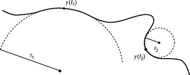
H. Steinhaus (1930) suggested an integral geometry-based method of estimating the length of a curve, which is still popular in stereology. Let γ be a plane Jordan curve that is rectifiable so that it has finite length L = ||γ||2 Let g (ψ) be the straight line through the origin that makes angle ψ with, for example, the positive x-axis. The orthogonal projection of γ onto this line can be regarded as a superposition of intervals, each of which is a projection of an arc of γ; see Figure 8.1 for an example. Let L(ψ) be the sum of the lengths of these intervals, and let ![]() be the mean of L(ψ) taken over all directions. From integral geometry, the following is known:
be the mean of L(ψ) taken over all directions. From integral geometry, the following is known:

FIGURE 8.1 Left: projection of a simple curve onto a line. Right: estimation of lengths of arcs by numbers of intersection points.
Here γ(t) = (x(t),y(t)) is assumed to be C(2)-regular: x(t) and y(t) have bounded second derivatives in a finite number of open intervals, so γ(t) is the union of a finite number of arcs with continuously turning tangents. On the basis of Equation 8.3, H. Steinhaus suggested measuring L(ψ) for n> 0 values of ψ equally spaced in the interval (0,2π) and taking the mean L of these values. He showed that the following is true if n is even and that these bounds are the best possible:
This equation gives a comparison of the mean ![]() on sampled angles and the mean
on sampled angles and the mean ![]() on continuous angles.
on continuous angles.
In numeric analysis, we usually estimate geometric properties of a curve in ![]() n from finitely many samples of the curve by fitting curves of known types to the samples and calculating the lengths of these approximating curves. Let γ : [0,1] →
n from finitely many samples of the curve by fitting curves of known types to the samples and calculating the lengths of these approximating curves. Let γ : [0,1] → ![]() n be a C(k)-regular parametric curve; our task is to estimate L(γ) from m + 1 points qi = γ(ti) on γ. This estimation is easiest when the tis are uniformly spaced (i.e.,
n be a C(k)-regular parametric curve; our task is to estimate L(γ) from m + 1 points qi = γ(ti) on γ. This estimation is easiest when the tis are uniformly spaced (i.e., ![]() [see Figure 8.2]). We will approximate γ with a curve
[see Figure 8.2]). We will approximate γ with a curve ![]() that is piecewise polynomial of some degree a ≥ 1.
that is piecewise polynomial of some degree a ≥ 1.

Theorem 8.1
Let γ be C(a+2) and ti = i/m. Then the tis determine a function ![]() , which is a piecewise degree-a polynomial such that the following is true, where a0 = 1 or 2 according to whether a is odd or even:
, which is a piecewise degree-a polynomial such that the following is true, where a0 = 1 or 2 according to whether a is odd or even:
![]() is called a Lagrange estimate of L(γ). We say that the tis are (ε, k)-uniformly sampled (ε ≥ 0 and k ≥ 1) iff there is a C(k) reparameterization φ : [0,1] → [0,1] such that the following is true:
is called a Lagrange estimate of L(γ). We say that the tis are (ε, k)-uniformly sampled (ε ≥ 0 and k ≥ 1) iff there is a C(k) reparameterization φ : [0,1] → [0,1] such that the following is true:
![]() can behave badly for (0,k)-uniform samplings, but for 0 <ε ≤ 1, we have the following:
can behave badly for (0,k)-uniform samplings, but for 0 <ε ≤ 1, we have the following:
Theorem 8.2
Let the tis be (ε, k)-uniformly sampled, where 0 <ε ≤ 1 and k ≥ 4. Then, for a = 2, we have the following:
In digital geometry, we must deal with digitization rather than sampling; pixel coordinates are known only to the accuracy imposed by the grid resolution. Piecewise linear curve approximation (a = 1) is usually preferred because of the simplicity of adding the lengths of line segments (see Chapter 10). However, Theorem 8.1 indicates that higher-order approximation may (!) have the potential for more accurate estimation.
8.1.3 Curvature
A Jordan curve is called smooth if it is continuously differentiable. Evidently, a polygon is not smooth, and a nonregular parameterization of a curve is not smooth at singular points. Curvature can be defined only at nonsingular points of a curve; in this section, we therefore assume a regular parameterization.
To define curvature, it is convenient to use the Frenet frame,1 which is a pair of orthogonal coordinate axes (see Figure 8.3) with the origin at a point p = γ(t) on the curve. One axis is defined by the unit tangent vector,

where ψ is the slope angle between the tangent and the positive x-axis. The other axis is defined by the unit normal vector:
n(t)=(–sin ψ(t),cos ψ(t))= −sin ψ(t)e1+cos ψ(t)e2
Evidently, 〈 t(t), n(t)〉e = 0. It is assumed that t(t) and n(t) define a right-handed coordinate system.
Figure 8.3 also illustrates the fact that l = L(t) is the arc length between the starting point γ(a) and the general point p = γ(t). As t increases, the changes in the tangent and normal are as follows:
The curvature of γ is its “rate of turn ” (i.e., the rate of change of ψ as p moves along γ).
p is called a convex point of γ if the curvature of γ at p is positive and a concave point if it is negative. Figure 8.4 shows on the left a positive point, on the right a negative point, and in the middle a point of inflection where the curvature changes sign. As Figure 8.4 shows, the situation at p can be approximated by measuring the distances between γ and the tangent to γ at p along equidistant lines that are perpendicular to the tangent. In Figure 8.4, positive distances are represented by bold line segments and negative distances by “hollow ” line segments. The area between the curve and the tangent line can be approximated by summing these distances; it is positive on the left, negative on the right, and zero in the middle, where the positive and negative distances cancel.

FIGURE 8.4 Three tangents to a curve. The curvature is positive on the left, has a zero crossing in the middle, and is negative on the right.
If an arc of γ is given explicitly as y = f(x), this definition evaluates to the following:

If γ is given explicitly in polar coordinates as r = f(η), we have the following:
Finally, in the general case of a parametric representation γ(t) = (x(t),y(t)), we have the following,
If we use the arc length parameterization, we have ![]() .
.
From Definition 8.1 and Equations 8.2 and 8.6, we have the following:
These two equations are called the Frenet formulae. If we use the arc length parameterization with unit speed v(l) = 1, the formulae simplify to the following:
For example, for a circle, we have γ(t) = (r cos t, r sin t), v(t) = r, and ![]() so that k(t) = 1/r by the first Frenet formula.
so that k(t) = 1/r by the first Frenet formula.
The absolute value of the curvature at p = γ(t) is equal to the inverse of the radius r(t) of the osculating circle at p, which is the largest circle tangent to γ on the concave side of p; see Figure 8.5. Note that we cannot have r(t)= 0, but r is infinite when p is on a straight line segment. In general, we have the following:
The sign of κ depends on whether γ is locally convex or concave at γ(t).
The curvature of a digital curve can be estimated using approximations to the tangent vector, estimated derivatives along the curve, or approximations to the osculating circle; see Chapter 10.
8.1.4 Angle
We saw in Section 3.1.3 that the angle η between two vectors can be expressed in terms of the scalar product of the vectors. In n-dimensional Euclidean space (n ≥ 2), we have the following:
Let two smooth curves γ1 = (x1,y1) and γ2 = (x2,y2) intersect at p = γ1(t1) = γ2(t2). Let the unit tangent vectors of γ1 at t = t1 and of γ2 at t = t2 be t1 and t2. The angle η between p1 and p2 at p satisfies the following, because ||t1||2 = ||t2||2 = 1:
Equation 3.7 shows that angular values can also be defined by weak scalar products; this generalizes the Euclidean space approach. See Section 3.3.3 for a discussion of angular values for grid-based metrics. Weak scalar products can also be defined for graph metrics on adjacency graphs.
Angles between digital curves can be estimated using approximations to their tangent vectors; see Chapter 10.
8.1.5 Area
A planar region R is a compact set in ![]() 2. Every compact is closed (and hence measurable, which means that it has a well-defined content) and bounded (so that its measure is finite); thus it is integrable. The area of R is given by the following:
2. Every compact is closed (and hence measurable, which means that it has a well-defined content) and bounded (so that its measure is finite); thus it is integrable. The area of R is given by the following:
Area is additive2; if R1 and R2 are planar regions that have disjoint interiors, we have A(R1 ∪ R2)= A(R1) + A(R2). This allows us to measure the area of a set by partitioning the set into (e.g., convex) subsets and adding the areas of these subsets.
Let T be a triangle pqr where p = (x1,y1), q = (x2,y2), and r = (x3,y3). Then we have the following:
where D(p,q,r) is the determinant:

Note that D(p, q, r) can be positive or negative; this can be used to define the orientation of the ordered triple (p,q,r). More generally, let P = <p1,p2,…,pn> be a simple polygon, n ≥ 3, and pi = (xi,yi). Then the following is true,
where po = pn and pn+1 = p1. Let the coordinate transformation u = u(x,y), v = v(x, y) map an integrable set R in the xy coordinate system into S in the uv-coordinate system, and let ux,uy,vx,vy be the partial derivatives of u and v with respect to x and y. Then the following is called the Jacobian matrix of the transformation:
Note that | J| = |uxvy – uyvx|. For example, for u = 5x2 + 3y and v = 6x2y + 2y2,we have ux(x,y)= 10x, uy(x,y) = 3, vx(x,y)= 12xy, and vy(x,y) = 6x2 + 4y.
The inner and outer Jordan digitizations can be used to estimate the area of a planar region. If S is a compact subset of ![]() 2, the areas
2, the areas ![]() and
and ![]() converge to the area A(S) as the grid resolution h →∞.
converge to the area A(S) as the grid resolution h →∞.
In Figure 8.6, S (upper left) is an unknown set; G (upper middle) is its Gauss digitization; and the upper right shows its inner and outer Jordan digitizations. The area of the relative convex hull (lower right) of the inner digitization with respect to the outer digitization (see Section 1.2.9) can also be used as an estimate of A(S). The lower row of the figure shows three other polygons with areas that could be used to estimate A(S). Theorems 2.2, 2.3, and 2.4 provide theoretic justifications of the multigrid convergence of these area estimators; their measurement bias is also important. Figure 8.7 shows how they differ from S for a fixed grid resolution. It can be shown experimentally that the inner Jordan digitization (lower left) leads to underestimation of the area, but the estimates based on the relative convex hull, the cardinality of the set of grid points, and the polygonal frontier defined by the midpoints of the invalid edges are “less biased.”

FIGURE 8.6 Upper row: unknown set S; Gauss digitization of S; and inner and outer approximations to S, which also show the convex hull of the inner approximation relative to the outer approximation. Lower row: 8-curve passing through the 4-border pixels; union of the 2-cells; and curve passing through the midpoints of the invalid edges.
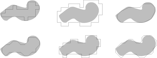
FIGURE 8.7 Visual comparison of an unknown set S with polygons that could be used to estimate its area, starting with inner and outer Jordan digitizations in the upper row and then following Figure 8.6.
8.1.6 Isothetic grid polygons
In this section, we discuss geometric properties of simple isothetic polygons Π with vertices that are grid points. Let f be the number of grid squares contained in Π,α0 the number of grid points in Π, and l the number of grid points on the frontier δΠ. By Pick ’s formula (see the comments following Theorem 4.10), we have the following:
When we trace the frontier (see Chapter 5) of a region in the frontier grid, the resulting polygonal chain does not necessarily circumscribe a single simple grid polygon. For example, in Figure 8.8 (right), the frontier of an 8-connected region in the picture grid circumscribes three simple polygons. In general, it circumscribes a sequence of simple isothetic grid polygons Π1,…,Πn (n ≥ 1). Because the area is additive, from Pick ’s formula (Equation 8.17) we have the following,
where L is the total length of the frontier (i.e., ![]() and
and ![]() is the number of grid points in
is the number of grid points in ![]() . To count α0, we can use discrete column-wise integration: start with α0 := 0;α0 := α0 + y for all p =(x, y) at the upper end of a run of object pixels in the y direction; and α0 := α0 – y + 1 for all p = (x,y) at the bottom of such a run. Figure 8.8 shows all of the local patterns that can occur in the frontier tracing, each with its corresponding increment, and also illustrates how the α0 values change during frontier tracing when we start at the uppermost-leftmost vertex and trace the frontier clockwise. In this example, we have α0 = 64 and L = 54 so that f = 36.
. To count α0, we can use discrete column-wise integration: start with α0 := 0;α0 := α0 + y for all p =(x, y) at the upper end of a run of object pixels in the y direction; and α0 := α0 – y + 1 for all p = (x,y) at the bottom of such a run. Figure 8.8 shows all of the local patterns that can occur in the frontier tracing, each with its corresponding increment, and also illustrates how the α0 values change during frontier tracing when we start at the uppermost-leftmost vertex and trace the frontier clockwise. In this example, we have α0 = 64 and L = 54 so that f = 36.

FIGURE 8.8 Left: local patterns used in discrete column-wise integration; right: an example of counting α0.
Finally, we prove a proposition (compare with Theorem 4.9) about the numbers of convex and concave vertex angles of a frontier of a simple isothetic grid polygon Π. We will use the same method in Section 8.3.7 to prove a theorem about the angles of isothetic simple grid polyhedra.
In the following discussion, we consider only the outer frontier of Π, which we assume is traversed clockwise. Inner frontiers (see Figure 8.9), which we assume are traversed counterclockwise, can be treated similarly. If three consecutive vertices pqr on the frontier are not collinear, we call the vertex at q convex if its vertex angle is π/2 and concave if it is 3π/2.

Proposition 8.1
Let ΠA and ΠC be the numbers of convex and concave angles of Π; then we have the following:
Proof For a single rectangle, we have ΠA = 4 and ΠC = 0. Any Π can be partitioned into a finite number of isothetic rectangles. Hence Π can be constructed by starting with a single isothetic rectangle and joining isothetic rectangles one at a time to an isothetic simple polygon. The four ways of performing the joins are shown in Figure 8.10.

In case (1), ΠA and ΠC remain unchanged; in case (2), both ΠA and ΠC increase by 1; and in cases (3) and (4), both ΠA and ΠC increase by 2. Hence ΠA through ΠC remain 4 throughout the process.
8.2 Space Curves and Arcs
A curve in ![]() n is a one-dimensional continuum; see Definition 7.2. For n = 3, we can use either of two analytic representations for a curve: two equations define a curve as the intersection of two surfaces, or a parameterization γ(t) = (x(t),y(t),z(t)), which also provides a direction and speed v(t). For example, the curve γ(t) = (a cost, a sint, bt), which is a circular helix that “winds around ” a cylindric surface, is characterized by a diameter 2a and a vertical distance 2πb; here a second surface that defines such a helix —together with the cylindric surface —is not uniquely defined. Changing b to –b changes the helix from “right-handed ” to “left-handed ” or vice versa.
n is a one-dimensional continuum; see Definition 7.2. For n = 3, we can use either of two analytic representations for a curve: two equations define a curve as the intersection of two surfaces, or a parameterization γ(t) = (x(t),y(t),z(t)), which also provides a direction and speed v(t). For example, the curve γ(t) = (a cost, a sint, bt), which is a circular helix that “winds around ” a cylindric surface, is characterized by a diameter 2a and a vertical distance 2πb; here a second surface that defines such a helix —together with the cylindric surface —is not uniquely defined. Changing b to –b changes the helix from “right-handed ” to “left-handed ” or vice versa.
When we use a parametric representation, we must also specify the domain of t, for example a ≤ t ≤ b.γ is smooth iff x(t),y(t), and z(t) are continuously differentiable. Analogously with Equation 8.1, the arc length of γ between the starting point γ(a) and the general point γ(t) is as follows:
If v(t) = 0,γ(t) is called a singular point. A point can be singular with respect to one parameterization but not with respect to another. A parameterization is called regular if it has no singular points. Unit speed v(t) = 1 can be achieved by using the arc length parameterization, which is regular.
For any regular parameterization of γ, we can define a unit tangent vector t at each point of γ. The curvature of γ is the absolute rate of change of direction of its tangent vector, where l = L(t) is arc length:
For the arc length parameterization γ(l), it follows that ![]() is the radius of(the circle of) curvature. As in the planar case, this is also called the radius of the osculating circle. On a straight segment of γ, we have κ = 0, and the radius of curvature becomes undefined (or infinite).
is the radius of(the circle of) curvature. As in the planar case, this is also called the radius of the osculating circle. On a straight segment of γ, we have κ = 0, and the radius of curvature becomes undefined (or infinite).
Any direction in the plane perpendicular to the tangent vector at a point p of γ is a normal direction to γ at p. A natural choice is ![]() , because
, because ![]() , so
, so ![]() is in this plane. The unit vector
is in this plane. The unit vector ![]() is called the principal normal. In accordance with Equation 8.19, we have the following:
is called the principal normal. In accordance with Equation 8.19, we have the following:
The cross product (vector product) b = t × n defines a third vector b called the binormal, which is orthogonal to both t and n. Let t = (t1,t2,t3) and n =(n1,n2,n3), and let the unit vectors in the coordinate directions be e1 = (1,0,0), e2 = (0,1,0), and e3 = (0,0,1); then the following is given:
b=(t2n3–t3n2)e1+(t3n1–t1n3)e2+(t1n2–t2n1)e3
t(t), n(t), and b(t) define an orthogonal coordinate system at γ(t) called the 3D Frenet frame.
The torsion of γ is defined by the following, where l = L(t) is arc length:
1/τ(t) is the radius of (the circle of) torsion. A curve is planar iff its torsion is identically zero; hence the torsion of γ can be thought of as measuring the departure of γ from planarity.
Estimation of arc length, curvature, and angle for 3D digital curves will be discussed in Chapter 10.
8.3 Surfaces and Solids
In Section 7.4, we gave a topologic definition and classification of surfaces. In this section, we discuss geometric properties of surfaces and of “solid ” objects.
8.3.1 Analytic representations
A surface can be represented analytically either by an equation f (x,y,z) = 0 or in parametric form. In this section, we will use a parametric representation: Γ(u, v) = (x(u,v),y(u,v),z(u,v)). We will assume that the functions x, y, and z have partial derivatives as follows and similarly for y and z:
Definition 8.2
A smooth surface patch Γ is defined by a simply connected compact set B ⊆ ![]() 2 and three functions x(u,v), y(u,v), and z(u,v), each of which is continuously differentiable for all (u,v) ∈ B, such that the following is true:
2 and three functions x(u,v), y(u,v), and z(u,v), each of which is continuously differentiable for all (u,v) ∈ B, such that the following is true:
We assume that two points (u,v) ∈ B never define the same point (x, y, z) of Γ (injectivity condition) and that the matrix of first derivatives has rank 2 for all (u,v) ∈ B :
If the other conditions are satisfied but the rank of the matrix is less than 2 at some points (u,v) ∈ B, we say that γ has singularities at those points.
A smooth surface patch Γ cannot be a Jordan surface, which must be homeomorphic to the surface of a sphere. The C(1) property of the functions x(u,v), y(u,v), and z(u,v) also allows no discontinuities in the derivatives; a polyhedral surface patch is not smooth.
As an example, consider the surface Γ of the sphere x2 + y2 + z2 – r2 = 0. A possible parameterization for this surface is as follows:
Γ(u,v)=(r cos u cos v,r cos u sin v,r sin u) where 0 < u <π and 0 < v < 2π
Here u is called the latitude angle and v is called the longitude angle. The sin and cos functions are continuously differentiable for all (u,v), and the matrix of first derivatives has rank 2. Note that this parameterization does not represent the entire surface; one semicircle joining the poles is not included. Definition 8.2 requires B to be compact; this can be achieved by using B = {(u,v):ε ≤ u ≤ π –ε Λε ≤ v ≤ 2π –ε} for some small ε> 0. In accordance with the wording latitude and longitude for u and v, the bounds on u, v mean that the Greenwich meridian (including the north and south poles) is removed. This is necessary in order to guarantee the injectivity condition of Definition 8.2.
As a second example, let B be a simply connected compact region in a plane Π. We can define a smooth surface patch Γ parallel to Π by taking x(u,v) = constant, y(u,v) = u, and z(u, v)= v. The matrix of partial derivatives has rank 2:

As a third example, let Γ be defined by the equation z = f (x, y) for (x, y) ∈ B ⊆ ![]() 2. Then Γ has the parameterization {(x,y,f (x,y)) :(x,y) ∈ B}. Such a Γ is called a Monge patch; it is smooth iff f is continuously differentiable for all (x, y) ∈ B.
2. Then Γ has the parameterization {(x,y,f (x,y)) :(x,y) ∈ B}. Such a Γ is called a Monge patch; it is smooth iff f is continuously differentiable for all (x, y) ∈ B.
8.3.2 Surface area
Let Γ have no singularities so that at least one of the subdeterminants given here is nonzero at each point of B:

The area of Γ is then defined as follows,
provided Γ is measurable (see Definition 8.4 and Theorem 8.3 on p. 286).
If Γ is a planar surface patch, we have the following,
so that the surface area measurement problem is reduced to a planar area measurement problem.
The definition of measurability of Γ is based on the triangulation of a bounded set B1 such that ![]() and such that the first derivatives of x(u,v), y(u,v), and z(u,v) exist and are continuous in
and such that the first derivatives of x(u,v), y(u,v), and z(u,v) exist and are continuous in ![]() (formally, x(u,v), y(u,v), and z(u,v) are functions in
(formally, x(u,v), y(u,v), and z(u,v) are functions in ![]() ).
).
In No. 108 of [696], it is shown that the angles η of the triangles in such a triangulation must satisfy η < 2π/3. This was proved independently by O. Hölder (p. 29 of [441]) in 1882, by G. Peano [806] in 1890, and by H.A. Schwarz [968] in 1890. We will now review the example given by H.A. Schwarz.
In 3D picture analysis, objects are often acquired slice by slice. The question arises whether surface area estimates can be based on triangulations that involve different slices (e.g., calculated by a marching cubes algorithm; see Section 8.4.2). It is also important that refining the acquisition process should result in more accurate estimates of surface area; see the concept of multigrid convergence in Section 2.4.3.
Example 8.1
Let a right circular cylinder of radius r and height h be cut by k − 1 planes (k ≥ 2) parallel to the bases of the cylinder, which segment the cylinder into k congruent parts. Construct a regular n-gon (n ≥ 3) in each of the k + 1 cross-sections (including the bases); see Figure 8.11, where n = 6. Rotate the n-gon by π/n between successive slices. Connect each edge of each n-gon to the vertex of each neighboring n-gon that is closest to the edge. This results in a triangulation Zk,n of the surface of the cylinder into 2kn congruent triangles that have the following total area:

As k and n go to infinity, the lengths of the edges of the triangles go to zero. However, the area of Zk,n does not converge to the surface area A(L) = 2πrh of the cylinder unless k/n2 goes to zero. If k/n2 converges to g> 0, A(Zk,n) converges to the following
k/n2 can even go to infinity (e.g., when k = n3); in that case, A(Zk,n) goes to infinity as well.
Note that this example uses sample points on the surface; such points are usually not available in digital geometry, so surface area estimates in digital geometry may be even less accurate. The example also shows that a method (approximation by n-gons) can work in one case (see Section 1.2.7 about the estimation of π) but not in another.
We now define a class of triangulations that satisfy the constraint η < 2π/3:
Definition 8.3
Let B1 ⊆ ![]() 2 be a simply connected compact set such that
2 be a simply connected compact set such that ![]() and let 0 <ω <π/3. A network Z of triangles that completely covers B1 is called a triangular subdivision of B1 with respect to B if it satisfies the following conditions:
and let 0 <ω <π/3. A network Z of triangles that completely covers B1 is called a triangular subdivision of B1 with respect to B if it satisfies the following conditions:
A triangular subdivision Z of B1 with respect to B defines a polyhedral approximation Γ (Z) of Γ by orthogonal projection of the vertices of Z onto3 Γ, and the adjacency relation between the vertices of Z defines an adjacency relation between these vertices on Γ. The surface area A(Γ (Z)) is defined to be the sum of the areas of the triangular faces of Γ(Z).
Definition 8.4
Suppose there exists a sequence Z1,Z2,Z3, … of triangular subdivisions of B1 with respect to B such that at→ 0, where at is the maximum length of any side of any triangle in Zt. This sequence defines a sequence of polyhedral approximations Γ(Z1),Γ(Z2), Γ(Z3), … of Γ that have well-defined surface areas AΓ(Z1)), AΓ(Z2)), AΓ(Z3)), …. We say that Γ is measurable if the following is bounded:
Theorem 8.3
If Γ is a measurable smooth surface patch, we have the following,
which is independent of the parameterization of Γ, where D1,D2, and D3 are the subdeterminants defined in Equation 8.22.
Let Γ be a Monge surface patch defined by z = f (x,y) for (x,y) in a closed bounded measurable set B ⊂ ![]() 2, where the first-order partial derivatives of f exist and are continuous on a set B1 such that
2, where the first-order partial derivatives of f exist and are continuous on a set B1 such that ![]() . By Theorem 8.3, the area of Γ = {(x,y,f (x,y)):(x,y) ∈ B} is as follows:
. By Theorem 8.3, the area of Γ = {(x,y,f (x,y)):(x,y) ∈ B} is as follows:
The vector (fx(x,y),fy(x,y)) is called the gradient of Γ at (x,y) ∈ B. Let np(x,y) = (–fx(x,y), – fy(x,y), 1) and nn(x,y) = (fx(x,y),fy(x,y), −1); these vectors are the normals to Γ at (x,y). Then we have the following:
This formula can be used to design surface area estimators for digital sets using estimated surface normals.
The formula in Theorem 8.3 can be rewritten in terms of the following expressions, which define the first fundamental form (E, F, G) of Γ:
This form satisfies both of the following conditions:
Chapter 11 will discuss the estimation of the surface area of a 3D digital object based on approximating its surface by, for example, planar surface patches. A 3D picture can be regarded as a sequence of 2D pictures, each of which is a digitization of a 2D cross-section of the scene. The inference of 3D properties from 2D cross-sections is studied in stereology using probability-theoretic models for the sampling processes involved; see Section 1.2.11. A general formula of stereology in traditional “stereologic notation ” is as follows,
where Vv is the volume of a solid K (in unit test volumes), AA is the area of K in test planes per unit test area, LL is the length of line intercepts with K in test lines per unit test line length, and Pp is the ratio between the number of points in K and the total number of test points. Equation 8.27 assumes that these measurements are statistically uniform. To estimate surface area, we can use the following identities,
where Sv is surface area per unit test volume, LA is the length of line elements per unit test area, PL is the number of points per unit test line length, Pv is the number of points per unit test volume, Lv is the length of line segments per unit test volume, and PA is the number of points per unit test area.
8.3.3 Example: an ellipsoid
To illustrate the difficulty of calculating surface area, we consider the example of an ellipsoid. Gauss, or outer and inner Jordan, digitizations (see Figure 8.12) of ellipsoids or combinations of ellipsoids (e.g., subtracting smaller ellipsoids from larger ones, thereby defining holes or cavities within the larger ellipsoids) provide useful data sets for testing 3D algorithms (e.g., for estimating surface area and comparing it with the correct value).
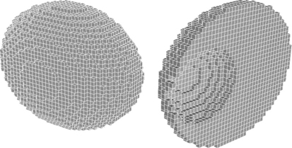
FIGURE 8.12 Left: a digitized ellipsoid. Right: a slice through a digitized ellipsoid from which a smaller ellipsoid that touches the larger ellipsoid at one surface point has been subtracted.
An ellipsoid is certainly an “elementary ” solid. Its surface area can be expressed by elementary analytic functions if two of its radii are equal (i.e., if it is an ellipsoid of revolution [216]). It was asserted in 1979 [494] that, “Except for the special cases of the sphere, the prolate spheroid, and the oblate spheroid, no closed form expression exists for the surface area of the ellipsoid. This situation arises because of the fact that it is impossible to carry out the integration in the expression for the surface area in closed form for the most general case of three unequal axes. In spite of the widespread use of the ellipsoid as a mathematical model and the extensive knowledge about the theory of curved surfaces and numeric integration, the problem of approximating the surface area of a triaxial ellipsoid does not appear to have been addressed.”
In fact, in 1825, A.M. Legendre (p. 352–359 in [640]) expressed the surface area of a general ellipsoid in terms of incomplete elliptical integrals (for an accessible reference, see [628]). If the ellipsoid is nearly spherical, Legendre ’s explicit formula is unsuitable for numerical computation, but a rapidly convergent series can be used.4 A simpler computation of the surface area of a general ellipsoid is due to G. Tee [498]; it is not limited to be an ellipsoid of revolution. This computation is given here next; it allows accurate area estimation independent of the parameters of the ellipsoid.
An ellipsoid Ea,b,c with semiaxes a, b, and c centered at the origin and with axes of symmetry along the coordinate axes has the following equation:
If two semiaxes are equal (e.g., b = c), Ea,b,c is generated by rotation around the x-axis of the halfellipse, with y ≥ 0:
The surface area A(Ea,b,b) is as follows, where u = x/a and q = 1 – b2/a2:
Therefore, we have the following:

The truncated power series shown here can be used if |q| ![]() 1:
1:
A(Ea,b,c) can be calculated using Equation 8.24. Without loss of generality, the coordinate axes can be chosen so that a ≥ b ≥ c. The surface z = f (x,y) of Ea,b,c satisfies the following conditions:
In the octant in which x, y, and z are all nonnegative, the surface area is as follows:

The integral with respect to y is as follows,


is Legendre ’s complete elliptical integral of the second kind.5 Hence, we have the following:
This expression can be evaluated numerically. Archimedes showed that, for a = b = c, the integrand is constant at π/2; see [1083]. As ![]() , the integrand converges to
, the integrand converges to ![]() , which has a singular derivative at s = 1. To get a smoother integrand, let u2 = 1 – s; then the following is true,
, which has a singular derivative at s = 1. To get a smoother integrand, let u2 = 1 – s; then the following is true,

where s = 1 – u2 and m (0 ≤ m ≤ 1) is as defined in Equation 8.29. The integral h(m) decreases from π/2 to 1 as m increases. The Arithmetic-Geometric Mean of C.F. Gauss is a very efficient tool for evaluating both h(m) and Legendre ’s complete elliptical integral k(m) of the first kind (see Milne-Thomson ’s Section 17.6 in [3]):

However, if m is very close to 1, the power series in m1 = 1 – m (p. 54 in [168]) should be used to evaluate k(m) for m < 1 and to evaluate h(m) for m ≤ 1.
The integrand with respect to u in Equation 8.30 is smooth enough for the integral to be evaluated by Romberg integration for c > 0. As ![]() , the ellipsoid converges to a two-sided elliptical lamina with surface area 2πab. Hence, for c/a
, the ellipsoid converges to a two-sided elliptical lamina with surface area 2πab. Hence, for c/a![]() 1, the area should be 2πab plus some terms in c/a.
1, the area should be 2πab plus some terms in c/a.
8.3.4 Gauss ’ definition of surface curvature
Let Γ be a smooth surface patch such that Γ(u,v) = (x(u,v),y(u,v),z(u,v)) and (u,v) ∈ B is not a singular point. Then Γu(u,v) = (xu(u,v),yu(u,v),zu(u,v)) and Γv (u,v) = (xv (u,v),yv (u,v),zv (u,v)) are tangent vectors to Γ at Γ(u,v). These vectors are not parallel; they therefore define a plane called the tangent plane to Γ at Γ(u, v) that contains all of the tangent vectors to Γ at Γ(u,v).
The cross product Γu(u,v) × Γv(u,v) defines a normal direction perpendicular to the tangent plane. The unit surface normal at Γ(u, v) is as follows:
The normal points inward or outward, depending on whether its sign is positive or negative.
The vector emanating from the origin in direction n(u, v) intersects the surface of the unit sphere at a point. This defines a mapping of Γ onto the unit sphere called the Gauss map of Γ. C.F. Gauss defined surface curvature based on this mapping; the unit sphere is therefore sometimes called the Gaussian sphere.
Let Uε (p) be a small neighborhood of a point p ∈ Γ defined by intersecting Γ with a sphere of radius ε> 0 centered at p. Then the following is a smooth surface patch on the unit sphere:
n(Uε(p))={n(u,v):Γ(u,v)∈Uε(p)}
Gauss originally defined the curvature of Γ at p as the ratio between the area of this patch and the area of Uε(p) as ε → 0:
Definition 8.5
(C.F. Gauss, 1828) The (historic) Gaussian curvature of a smooth surface patch Γ at p = Γ(u,v) is as follows:
For numeric calculations, it is usually easier to replace the circular U-neighborhoods with rectangular neighborhoods. A point on the Gaussian sphere is specified by its longitude ξ and latitude η. Let δR be the (“rectangular ”) surface patch on the Gaussian sphere between ξ and ξ + δξ and between η and η + δη; thus A(δR) = δξ δη cos η. Let δΓ(u,v) be the patch of Γ around Γ(u,v) that defines δR. Then we have the following:
For example, a sphere of radius r> 0 has constant Gaussian curvature 1/r2.
In computer vision, G(ξ,η) = 1/kG(u,v) is called the Gaussian image of Γ; it is a “labeled ” Gauss map. If kG(u,v) = 0 (e.g., if Γ is locally planar at Γ(u,v)), G has a point impulse at (ξ,η) (defined by the surface normal at Γ(u,v)); the impulse is “labeled ” by the surface area that contributes to the impulse.
A finite convex polyhedron that has n> 0 faces has a Gaussian image that consists of n point impulses, each labeled by the area of the corresponding face. H. Minkowski has shown that convex polyhedra are determined up to translation by their face areas and normals; hence the labeled Gaussian image determines a convex polyhedron up to translation.
As an example of the calculation of Gaussian curvature, consider again the ellipsoid Ea,b,c defined by the following:
Γ(Φ,ψ)=(a cosψ cosΦ, b sinψ cosΦ, c sinΦ)
(see Figure 8.13 for the definitions of the angles Φ and ψ). Here the Gaussian curvature is as follows,

and the Gaussian image is as follows, where ξ and η are longitude and latitude on the Gaussian sphere:
Two smooth surface patches Γ1 and Γ2 are called isometric iff there is a one-to-one mapping ϕ from Γ1 onto Γ2 such that ϕ and ϕ−1 are both differentiable and ϕ maps any smooth arc in Γ1 onto a smooth arc in Γ2 of the same length. It is proved in differential geometry that two smooth surface patches are isometric iff they have identical first fundamental forms (E, F, G).
A local isometry ϕ from Γ1 onto Γ2 is a one-to-one differentiable function such that, for all p ∈ Γ1, there exist neighborhoods U(p) in Γ1 and U(ϕ(p)) in Γ2 such that ϕ is an isometry between the neighborhoods. For example, the surface of an infinite cylinder is locally isometric to a plane.
This theorem points out a limitation of the historic Gaussian curvature. We are usually interested in distinguishing between the local curvature of a plane (a planar point) and that of a cylinder (a parabolic point), but they are not distinguishable when the historic definition is used. Also, the historic Gaussian curvature is always nonnegative; it does not allow us to distinguish between the local curvature of an elliptical surface patch (an elliptic point) and that of a hyperbolic surface patch (a hyperbolic point). To overcome these limitations, differential geometry has introduced other measures of surface curvature (e.g., based on pairs of curves lying on the surface patch and intersecting at the given point). (The curvature of a space curve was defined in Section 8.2.) These measures will be defined in the next section.
8.3.5 Principal, Gaussian, and mean surface curvature
Let Γ be a Monge patch defined by z = f (x1,x2) on a planar region B, where f is in C(2)(B), so that it is twice continuously differentiable for all (x1,x2) ∈ B and therefore satisfies the integrability condition:
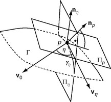
We calculate the surface curvature at p ∈ Γ using arcs Γ1 and Γ2 that are contained in Γ, pass through p, and are not parallel in a neighborhood of p. Let t1 and t2 be the tangent vectors to Γ1 and Γ2 at p. These vectors span the tangent plane Πρ to Γ at p. We assume angular orientations 0 ≤η < π in Πρ (a halfcircle centered at p).
The surface normal np at p is orthogonal to Πρ and collinear with the cross product t1 × t2. Let Πη be a plane that contains np and has orientation η; see Figure 8.14. Πη makes a dihedral angle η with Π0 and cuts Γ in an arc γη. (Πη may cut Γ in several arcs or curves, but we consider only the one that contains p.) Let tη, nη, and κη be the tangent, normal, and curvature of γη at p.κη is the normal curvature of any arc γ ⊂ Γ ∩ Πη at p that is incident with p. For example, take f to be the constant function with a value of 0 everywhere. Then the Monge patch is part of the horizontal plane through o = (0,0,0) in ![]() 3. Any γη is a straight line segment in the plane that is incident with o; we have κη = 0 and tη = γη. If we take f to be a “cap ” of a sphere centered at its north pole p,γη is a segment of a great circle on the sphere, nη is incident with the straight line passing through p and the center of the sphere, and κη = 1/r where r is the radius of the sphere.
3. Any γη is a straight line segment in the plane that is incident with o; we have κη = 0 and tη = γη. If we take f to be a “cap ” of a sphere centered at its north pole p,γη is a segment of a great circle on the sphere, nη is incident with the straight line passing through p and the center of the sphere, and κη = 1/r where r is the radius of the sphere.
The characteristic polynomial p of an n × n matrix A is defined as p(λ) = det(A –λI) = (–λ)n + … + det(A), where I is the n × n identity matrix. According to the Cayley–Hamilton Theorem [311], p(A) = 0. The eigenvalues λi of an n × n matrix A are the n roots of its characteristic equation det (A –λI) = 0.
Let v be a unit vector in Πp. The negative derivative –Dvn of the unit normal vector field n of a surface, which is regarded as a linear map from Πp to itself, is called the shape operator (or Weingarten map or second fundamental tensor) of the surface. Let Mp be the Weingarten map in matrix representation at p (with respect to any orthonormal basis in Πp), and let λ1 and λ2 be the eigenvalues of the 2 × 2 matrix Mp. Note that these eigenvalues do not depend on the choice of orthonormal basis in Πp.
It is proved in differential geometry [1014] that the absolute value of the Gaussian curvature is equal to the historic Gaussian curvature of Definition 8.5. The mean curvature is equal to (κη(p) + Kη+π/2(p)/)2 for any η ∈ [0,π).
In the case of a Monge patch, it is natural to choose b1 = (1,0, fx1) and b2 = (0,1,fx2) as basis elements for Πp; they are the images of the usual basis e1 = (1,0) and e2 = (0,1) of ![]() 2 under differentiation of the Monge patch. We then calculate the following matrix of inner products,
2 under differentiation of the Monge patch. We then calculate the following matrix of inner products,

which unfortunately is not the matrix Mp of the Weingarten map with respect to the basis {b1, b2}, because the latter is not necessarily orthonormal. The relationship between Pp and Mp is explained in [1014] (at the end of p. 50 of Volume 3),
where Gp is the metric tensor of Γ at p and we use the fact that Gp and Pp are symmetric matrices:
The following 2 × 2 matrix is called the Hessian matrix of Γ6:
The Monge patch satisfies the integrability condition a12 = a21 (i.e., its Hessian matrix is also symmetric).

Mp has a quadratic characteristic equation with two eigenvalues λ1 and λ2 at any surface point p. These eigenvalues define a pair of orthogonal eigenvectors v1 and v2 that satisfy the equations Mpv1 = λ1v1 and Mpv2 = λ2v2. By the symmetry of Mp (i.e., ![]() ), we have the following:
), we have the following:

It follows that λ1 ≠ λ2 implies 〈v1, v2〉 = 0, so v1 and v2 are orthogonal. (Sometimes,λ1 = λ2 [e.g., for a planar patch or a patch on a sphere]. In such cases, v1 and v2 are chosen as an arbitrary orthonormal pair of basis elements of Πp.) Let η = 0 be the direction of v1 or v2 in Πp (i.e., either λ1 or λ2 is κ0(p)).
Now let w1 and w2 be any two orthogonal vectors that span the tangent plane Πp to Γ at p (i.e., they are tangent vectors that define normal curvatures in directions η and η +π/2). Then the Euler formula
allows us to calculate the normal curvature κη (p) in any direction η at p from the principal curvatures λ1 and λ2 and the angle η.
Chapter 11 will discuss the estimation of mean surface curvature based on digital approximations to the surface. We can locally estimate the tangent plane Πp and thus the normal np at any point p on Γ (see Figure 8.14). We can also cut Γ at p by a plane Πc in some direction (e.g., parallel to the xz-plane at the y-coordinate of p). The intersection of Πc with Γ defines an arc γc in the neighborhood of p, and we can estimate the curvature κc of γc at p. However, we cannot assume that Πc is incident with the surface normal np at p. Let nc be the principal normal of γc at p. A theorem of Meusnier7 [727] tells us that the normal curvature κη in any direction η is related to the curvature κc and the normals np and nc by the following:
By estimating two normal curvatures κη and κη+π/2, we can estimate the mean curvature.
8.3.6 Volume
Let K ⊂ ![]() 3 be a compact set and f (x, y, z) a function such that 0 ≤ f (x, y,z) ≤ 1 for all (x, y, z) ∈ K. f (x, y, z) can be regarded as the “density ” of K at p =(x, y, z) ∈ K. The following integral defines the volume of f on K:
3 be a compact set and f (x, y, z) a function such that 0 ≤ f (x, y,z) ≤ 1 for all (x, y, z) ∈ K. f (x, y, z) can be regarded as the “density ” of K at p =(x, y, z) ∈ K. The following integral defines the volume of f on K:

If f (x,y,z) = 1 iff (x,y,z) ∈ K, I is the volume V(K). K is integrable iff it has a well-defined and finite volume. Every compact set is integrable.
Section 2.3.2 described Jordan ’s method of estimating the volume of a set using its inner and outer digitizations. It estimates the (Jordan) volume V(S) of S by its inner or outer volume, provided that these volumes converge to the same limit as the grid constant goes to zero.
Grid-based studies by Jordan and Peano initiated the field of combinatorial geometry (the geometry of numbers; see Section 1.2.8). A fundamental theorem of H. Minkowski says that a convex subset of ![]() n that is symmetric about o = (0,…,0) (i.e., if p is in the set so is – p) and that has a volume of at least 2n contains at least two grid points in addition to o.
n that is symmetric about o = (0,…,0) (i.e., if p is in the set so is – p) and that has a volume of at least 2n contains at least two grid points in addition to o.
Cavalieri ’s Principle8 [1031] is often used for area or volume estimation. Let R1 and R2 be two 2D regions that lie between two parallel lines Γ1 and Γ2. Suppose any line between Γ1 and Γ2 and parallel to them cuts R1 and R2 into straight line segments of equal (total) length; then R1 and R2 have equal area. Similarly, let R1 and R2 be two solids that lie between two parallel planes. If any plane between the two planes and parallel to them cuts the solids in regions of equal (total) area, then the solids have equal volume.
Estimating the volume of a digital set by counting voxels is justified by Cavalieri ’s Principle and by Jordan ’s method of volume measurement. Volume estimation can also be based on polyhedral approximation (as in the use of polygonal approximation for area estimation that was discussed at the end of Section 8.1.5) or on integral-geometry-based methods. For the latter approach, we briefly state a few basic equations.
Let Br = {p ∈ ![]() n : ||p||e ≤ r} be the n-dimensional ball of radius r> 0 around the origin, let M ⊂
n : ||p||e ≤ r} be the n-dimensional ball of radius r> 0 around the origin, let M ⊂ ![]() n, and let Mρ = M
n, and let Mρ = M ![]() Br be the Minkowski sum of M and Br. An oval is a bounded closed convex subset of
Br be the Minkowski sum of M and Br. An oval is a bounded closed convex subset of ![]() n. For example, if n = 1, M is a straight segment, and L(Mr) = L(M) + 2r. Let M ⊂
n. For example, if n = 1, M is a straight segment, and L(Mr) = L(M) + 2r. Let M ⊂ ![]() 2 be an oval with A(M) > 0; then we have the following:
2 be an oval with A(M) > 0; then we have the following:
If M ⊂ ![]() 3 is an oval with V(M) > 0, then the following is true, where
3 is an oval with V(M) > 0, then the following is true, where ![]() is the mean width of the oval M:
is the mean width of the oval M:
Both equations follow from Steiner ’s formula; see page 220 in [958]. The volume determines the surface area:
The mean width of a simple convex polyhedron M that has α1 edges is given by the following,
where li is the length of the ith edge ei and αi is the angle between the normals of the faces that intersect in ei. For the general case (i.e., the mean width of an arbitrary oval), see [958].
![]() is also called the mean curvature M(M) of the oval M. The total curvature C(M) is 4π for all ovals of nonzero volume. In general, these properties are defined by the following:
is also called the mean curvature M(M) of the oval M. The total curvature C(M) is 4π for all ovals of nonzero volume. In general, these properties are defined by the following:
Equation 8.33 becomes the following:
Steiner ’s formula also allows us to conclude the following (for an oval M ⊂ ![]() 3):
3):
Equations 1.10 and 1.11 also deal with ovals in ![]() 3.
3.
8.3.7 Isothetic polyhedra
Sections 5.2.2 and 5.2.3 discussed combinatorial topology for incidence pseudographs, and Section 5.3 discussed it in detail for regular infinite incidence pseudographs. The results can be interpreted as counting formulas for properties of isothetic grid polygons or polyhedra.
Let Π be the simply connected union of a finite set of 6-connected simple polyhedra. The volume α3 of Π can be calculated using formulas given in Section 5.3.2 (e.g., on the values α0 and b03 and the constants a03 = a30 = 8). b03 can be calculated during frontier tracing, and α0 can be calculated using discrete column-wise integration as in Section 8.1.6. Section 5.3.2 also provides ways of calculating α3 based on the values α1 and b13 and the constants a13 = 4 and a31 = 12 or on the values α2 and b23 and the constants a23 = 2 and a32 = 6.
We now derive a result about the angles of isothetic simple grid polyhedra. The counting formulas in Section 5.3 are formulas for isothetic simple grid polyhedra defined by unions of cells. The angle formula given in this section is based on a geometric construction, unlike the purely combinatorial approach used in Section 5.3. It also provides a method of defining topologic invariants that distinguish inner surfaces from outer surfaces.
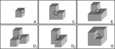
There are six kinds of angles in an isothetic simple polyhedron; see Figure 8.15. These angles will be referred to as being of types A, C, D1, D2, E, and G, respectively.
Theorem 8.6
Let Π be an isothetic simple polyhedron, and let ΠA, ΠC, ΠD1, ΠD2, ΠE, and ΠG be the numbers of angles of Π of types A, C, D1, D2, E, and G. Then we have the following:
T=(ΠA+ΠG)–(ΠC+ΠE)−2(ΠD1+ΠD2) = 8
Proof Π can be obtained by a finite sequence of joins of a simple isothetic polyhedron Π1 to a simple isothetic polyhedron Π2 in which a face P2 of Π2 is brought into coincidence with a subset of a face P1 of Π1. We can start the process with two isothetic rectangular parallelepipeds for which ΠA = 8 and all the other Πs are zero; thus these parallelepipeds satisfy the formula. At each step of the joining process Π1 and Π2 can have only A and C angles on their merging faces P1 and P2. By Proposition 8.1, the number of A-angles on P2 is always four greater than the number of C-angles. (P2 is a subset of P1; this excludes joining a C-angle on P2 with an A-angle on P1 or joining a C-angle on P2 with a point on an edge of P1.) Hence there are only six types of joinings, as shown in Figure 8.16:

i. an A-angle on P2 is joined with an A-angle on P1;
ii. an A-angle on P2 is joined with a C-angle on P1;
iii. an A-angle on P2 is joined with a point on an edge of P1;
iv. an A-angle on P2 is joined with an interior point of P1;
We can assume that Theorem 8.6 is valid for Π1 and Π2. Thus, before the joining operation, the total count for the two polyhedra is T = 16. We will now prove that T = 8 after the joining operation.
In case (i), an A-angle of Π1 and an A-angle of Π2 are lost; this decreases T by 2. In case (ii), a C-angle of Π1 and an A-angle of Π2 are lost, but the union gains a D1- or D2-angle, so T decreases by 2. In case (iii) an A-angle of Π2 is lost, but the union gains a C-angle, so T decreases by 2. In case (iv), an A-angle of Π2 is lost, but the union gains an E-angle, so T decreases by 2. In case (v), a C-angle of Π1 and a C-angle of Π2 are lost; this increases T by 2. In case (vi), a C-angle of Π2 is lost, but the union gains a G-angle so T increases by 2.
In summary, the four joinings of A-angles decrease T by 2, and the two joinings of C-angles increase T by 2. The number of A-angles on P2 is always four more than the number of C-angles; hence, after we perform the joining operations that involve all of the A- and C-angles of P2, we have T = 8.
The formulas in Proposition 8.1 and Theorem 7.13 are both useful for analyzing isothetic frontiers. In a 2D binary picture, an isothetic frontier is inner (the frontier of a union of proper holes) or outer, depending on whether Πv – ΠC < 0 or > 0. In a 3D binary picture, there are dualities between angles of types A and G, C and E, D1 and D1, and D2 and D2. Thus T = 8 whether we consider the surface as being the outer frontier of a simple polyhedron or an inner frontier of a proper polyhedral hole. However, we can use other quantities to distinguish between inner and outer frontiers; for example, ΠA – ΠG is negative for an inner frontier and positive for an outer frontier. The quantity T is also of practical interest; for example, it provides a test for whether the entire surface of an isothetic polyhedron has been traced. The six angle counts can also be used as shape descriptors.
8.4 Surface Tracing and Approximation
In Section 5.4.4, we briefly discussed the use of the FILL procedure to trace the 3D frontier of a simply connected region. In Section 8.4.1, we will describe a more efficient frontier tracing algorithm. In Section 8.4.2, we will describe a “marching cubes ” algorithm that approximates the frontier of a region by constructing a triangulation “between ” the border and coborder of the region.
8.4.1 The Artzy-Herman algorithm
The frontier of a 1- or 0-region of voxels splits in general into frontiers of a finite number of 2-regions; we will consider only 2-regions here. The FILL procedure discussed in Section 5.4.4 does not attempt to minimize the number of accesses to frontier faces to determine whether they have already been labeled; it is therefore also applicable to 0- or 1-regions. In a 2-region, any frontier face is edge-adjacent to exactly four9 other frontier faces; hence FILL makes at most four visits to each frontier face, including the first visit, when the face is labeled. The algorithm described in this section requires at most two visits to each face, including the first visit.
Let [F, A] be the undirected graph in which each node represents a frontier face of a closed 2-region M of voxels in the 3D incidence grid ![]() 3. We call two nodes f1 and f2 adjacent (f1 Af2) iff they are 1-adjacent in
3. We call two nodes f1 and f2 adjacent (f1 Af2) iff they are 1-adjacent in ![]() 3. Each f ∈ M is incident with one 3-cell I(f) in M and with one 3-cell O(f) in
3. Each f ∈ M is incident with one 3-cell I(f) in M and with one 3-cell O(f) in ![]() . Evidently, f1Af2 iff O(f1) = O(f2) (so that I(f1) and I(f2) are 1-adjacent) or O(f1) and O(f2) are 2-adjacent (so that I(f1) and I(f2) are also 2-adjacent) or O(f1) and O(f2) are both 2-adjacent to the same 3-cell in
. Evidently, f1Af2 iff O(f1) = O(f2) (so that I(f1) and I(f2) are 1-adjacent) or O(f1) and O(f2) are 2-adjacent (so that I(f1) and I(f2) are also 2-adjacent) or O(f1) and O(f2) are both 2-adjacent to the same 3-cell in ![]() (i.e., I(f1) = I(f2)). It follows that each node in [F, A] has degree 4.
(i.e., I(f1) = I(f2)). It follows that each node in [F, A] has degree 4.
Let I(f) be the 3-cell shown in Figure 8.17. In the graph representing the faces of I(f), there are three circuits, each of which is parallel to one of the coordinate planes. Each face has two outgoing and two incoming edges; each of these edges goes from one face to another by “crossing ” a 1-cell (grid edge). Each grid edge in the frontier of M is incident with exactly two frontier faces of M. If we start at any face f in the frontier of M, the two outgoing edges of f on I (f) point to two frontier
ALGORITHM 8.1 The Artzy-Herman algorithm for tracing all faces of a 3D frontier.

faces called the out-faces of f, and the two incoming edges are outgoing edges of two in-faces of f. The frontier tracing algorithm makes use of this directed graph structure (Algorithm 8.1). We accumulate all of the frontier faces of M in the list F. The queue Q implies a breadth-first access order; using a stack instead implies a depth-first access order. We can return to a face at most twice; the second copy of f0 on L is removed when we enter Step 2.a.i. for the first time.
8.4.2 Marching cubes
A set of voxels in a 3D picture P is supposed to be a representation (e.g., a Gauss digitization) of an unknown 3D object with an unknown surface. We choose a threshold T (0 < T ≤ Gmax) to define object voxels (P (p) ≥ T) and nonobject voxels (P (p) < T). The voxels of P at each z-coordinate define a 2D picture called a layer. We scan each layer of P to detect border voxels, which can be combined in successive layers to define triangular faces of the border [1141]. A marching cubes algorithm [667] uses eight voxels (a 2 × 2 × 2 block) on two successive layers of P to define triangles that approximate the unknown surface. These triangles are chosen by analyzing how the unknown surface could intersect the 2 × 2 × 2 block. The surface is assumed to intersect each grid edge (between two neighboring voxels) at most once. It follows that it can intersect a 2 × 2 × 2 block in 28 = 256 ways. The differences between T and the voxel values can be used to estimate the intersection points with grid edges. As a default, we assume that all edges are intersected at their midpoints.
Figure 8.18 illustrates situations that do not lead to unique triangulations. A marching cubes algorithm assumes that the 2 × 2 × 2 voxel configurations are mapped into possible triangulations by a look-up table. The 256 eight-voxel configurations can be reduced modulo rotations and symmetries. This leads to one homogeneous configuration (all eight voxels are inside or outside the object), which produces no triangle, and 14 other cases. Figure 8.19 shows a look-up table that specifies one triangulation for each of the 14 configurations. The union of the triangulations defines an isosurface for P that depends on the threshold T and the look-up table.


FIGURE 8.19 The 15 marching cubes configurations of [667].
Look-up tables occasionally produce isosurfaces that have holes. This happens if adjacent eight-voxel configurations produce “nonmatching ” triangles. The resulting isosurface has an acyclic vertex with a star (the set of triangles incident with it) that is not a cycle of triangles. Figure 8.20 shows an example that gives rise to about 1% acyclic vertices, depending on the threshold used. In this example, a 23-case look-up table was used; there were two choices for 8 of the 14 nontrivial cases.

FIGURE 8.20 Left: isosurface generated by a marching cubes algorithm (astrocytes in brain tissue). A 3D picture (256 × 256 × 51 voxels) was mapped into an isosurface defined by 407,216 vertices of generated triangles. Right: the isosurface after vertex reduction; it has only about 40% as many vertices as the isosurface shown on the left.
In Figure 8.20, a large number of triangles were generated. Reduction algorithms10 have been designed to decrease the number of triangles (e.g., by merging triangles that have almost identical normals).
8.4.3 Local and global polyhedrization
A solid Θ is a set in E3 with a frontier that is a closed, bounded, measurable, hole-free surface (see Chapter 7). A digitization of Θ in a grid with resolution h is a finite union digh(Θ) of 3-cells. A digital surface S is the frontier ![]() of such a set; it can be regarded as a 2D complex of 0-, 1-, and 2-cells or as a set of frontier faces. Note that S is an isothetic polyhedral surface.
of such a set; it can be regarded as a 2D complex of 0-, 1-, and 2-cells or as a set of frontier faces. Note that S is an isothetic polyhedral surface.
Θ can be magnified by a factor h> 0 (see Section 2.3.2) and digitization can be limited to a grid that has grid constant 1. Alternatively, Θ can be kept at its original size, but digitization can be done on a grid of resolution h> 0 (grid constant θ = 1/h). The first approach was preferred by Jordan and Minkowski; it has the advantage that the calculation of surface area involves only integer arithmetic and is therefore preferable in implementations. The second approach is common in numeric analysis; we will use it in multigrid convergence studies (following Definition 2.10).
Polyhedrization maps a digital surface S into a finite set of polygonal faces in E3 but does not always provide a simple polyhedral approximation of the (unknown) surface ![]() . For example, a triangulation produced by a marching cubes algorithm may not be hole-free and so may not be the surface of a simple polyhedron.
. For example, a triangulation produced by a marching cubes algorithm may not be hole-free and so may not be the surface of a simple polyhedron.
For each polygon Π of a polyhedrization of S, there exists a subset Ah (Π) of S such that Π depends only on Ah(Π); if SAh,(Π) is modified in any way into another digital surface, its polyhedrization still contains Π. Ah (Π) is called the ball of influence of Π. Because a polyhedrization of S contains only finitely many Πs, the set of radii of these balls of influence has a maximum value R(h, S).
The frontier faces of a simply 2-connected region (e.g., visited by the Artzy-Herman traversal algorithm) define a polyhedrization with constant ![]() . The marching cubes algorithm is a polyhedrization method with constant
. The marching cubes algorithm is a polyhedrization method with constant ![]() .
.
Definition 8.7 can be applied to other methods or properties that involve measurements in a metric space. Digital straight line segment (DSS) methods (as discussed in Chapters 9 and 10) are global methods. All of the methods of digitization defined in Chapter 2 are local methods.
8.5 Exercises
1. Give a parametric representation x = x(t), y = y(t) for the parabola defined by the equation y2 = 4ax. What is the domain of the parameter t? Do the same for the ellipse x2/a2 + y2/b2 = 1.
2. Calculate the curvature κ(t) of the parabola and ellipse defined in Exercise 8.1. (Hint: Apply one of the Frenet formulae.)
3. Let < p1,…,pn > be a simple polygon, and let ni be the unit normal of the side pipi+1 (1 ≤ i ≤ n). Let vi = || pi pi+1||2ni (where pn+1 = p1) be the normal weighted by the length of the side. Prove that v1 + … + vn is the zero vector (0,0).
4. Prove that, if the vectors defined in Exercise 3 are the same for two convex simple polygons, they must differ by a translation.
5. Show that the determinant D(p,q,r) in Equation 8.14 can be calculated using only two multiplications (and several additions/subtractions).
6. The following figure shows a unit square S0 in the upper left corner. Delete an “open cross ” from S0 as shown in the upper right corner; this results in a disconnected set S1 of four squares. Repeat this process for each resulting square to obtain a set S2 composed of 16 squares, a set S3 composed of 64 squares, and so on. Note that each Sn is a closed set and consists of a finite number of squares. Continue the process to infinity; recall that the family of closed sets is closed under arbitrary intersections. What is the area of the limiting set S0 ∩ S1 ∩ S2…?

7. Prove the area formula in Equation 8.15 for simple polygons.
8. Let D be a planar disk of radius a> 0 centered at the origin. What is the equation of D in polar coordinates x = r cos φ and y = r sin φ? What are the Jacobian matrix and Jacobians of this coordinate transformation?
9. Prove that a sphere of radius r> 0 has constant Gaussian curvature 1/r2.
10. The vector representation in Exercises 3 and 4 can be generalized to simple polyhedra: vi = A(Fi)ni where the Fis are the faces of the polyhedron and ni is the unit normal to Fi. Prove that v1 + … + vn is the zero vector (0,0,0).
11. Define cylindric coordinates x = r cos φ, y = r sin φ, and z = z and spheric coordinates x = r sin ψ cos φ, y = r sin ψsin φ, and z = r cos ψ. What are the Jacobian matrices and Jacobians of these coordinate transformations?
12. The characteristic polynomial of a general 2 × 2 matrix A is p(λ) = det(A –λI) = λ2 – (a11 + a22)λ + (a11a22 – a12a21). Prove that p(A)= A2 – (a11 + a22)A + (a11a22 – a12a21) I = 0, where I and 0 are the 2 × 2 identity and null matrices. (This proves the case n = 2 of the Cayley-Hamilton Theorem.)
13. Let S be a connected polygonal region that has b grid points on its n borders and i grid points in its interior. Prove that the area of S is ![]() .
.
8.6 Commented Bibliography
The geometry of curves and surfaces is treated in many textbooks, for example, [249, 781]. The Steinhaus method was proposed in [1022]. For parameter estimation of digital curves, see [1156]; for estimation of normals, see [751]. Higher-order approximations of curves (Theorems 8.1 and 8.2) were used for length estimation in [778, 779]. [704] gives a comprehensive review of methods of estimating curvature, including methods using vector algebra, which were not discussed in Section 8.1.3; see also [595].
The material in Sections 8.3.1 and 8.3.3 partially follows [498, 696]. Example 8.1 was published in [968] in 1890 and is also given in [696]. Theorem 8.3 was proved in [696]. For the study of surfaces in materials science, see [72, 147].
The Teorema Egregium was published by C.F. Gauss in [357]. Examples of the calculation of Gaussian curvature, including the formulas for the ellipsoid given in Section 8.3.4, are given in [971]. Theorem 8.4 is proved in [781, 1014]. For a proof of the Theorem of Meusnier, see [1014]. The application of basic theorems of differential geometry to digital geometry is discussed in [630].
For results about volumes of solids in the geometry of numbers, see [733, 842, 960]. The fundamental formulas about the content of “parallel bodies ” Mr (see the 2D and 3D formulas, Equations 8.32 and 8.33, and Section 1.2.11) are due to J. Steiner [1020]; due to Minkowski, they are of central importance in the theory of convex bodies today. G. Pick gave a formula for the area of not necessarily simply connected grid polygons in [816]. For applications of his formula to simple grid polygons in digital geometry, see, for example, [605, 877, 952, 1107]. The effect of ratio-based digitization (i.e., taking the percentage of the 2-cell occupied by the set into account) on area estimation using pixel counts was studied in [398]. For stereology, see [1079]. Cavalieri ’s Principle was published in 1635 in [166]. Equation 8.34 is from [964]. For integral geometry and geometric or grid inequalities for measures such as volume or surface area, see [98, 152, 393, 413, 746, 788, 963, 965, 1021].
Simpler and more efficient algorithms often exist for isothetic objects; see, for example, [1128]. Such objects can be regarded as boundaries of cell complexes [1005], and they often allow combinatorial approaches (see, for example, [226] about the visibility of isothetic rectangles). Isothetic polygons and polyhedra also have applications to VLSI (Very Large Scale Integration) layout, database design, computational morphology, stock cutting, and partitioning problems [227, 801]. Sections 8.1.6 and 8.3.7 review [1149].
The Artzy-Herman algorithm was published in 1981 [48]; see the preface of [430] for its history. For a proof that this algorithm always generates a 1-cycle (see Section 6.4.5) of faces, see [429]; [433] is an earlier version that contains a shorter proof. A modified algorithm for surface traversal of 26-connected regions is discussed in [809]. For other surface traversal algorithms, see [143, 582, 828, 1077].
Topologic ambiguities in local 3D surface approximation techniques such as the marching cubes look-up tables are discussed, for example, in [775]. The 23-case look-up table in Figure 8.20 was published in [1126]. For vertex reduction, see, for example, [776, 967]. Marching cubes algorithms are sometimes (inaccurately) used as a generic name for methods of level surface extraction from gridded data. A marching cubes algorithm is easy to implement and will be used in Chapter 12 to illustrate a failure of local methods to correctly estimate surface area. Bilinear interpolation on frontier faces, or trilinear interpolation on border voxels, provides topologically correct surface approximations. Recent algorithms (e.g., adaptive skeleton climbing [821], triangulation by ear clipping [292]), are based on digital geometry, topology, and multiresolution concepts and avoid [291] expensive postprocessing for triangle reduction, which is typically necessary with marching cubes algorithms.
[495] discusses simplicial surface constructions on the boundary (i.e., “between the border and coborder ”) of a 3D set of voxels. The surface of the resulting combinatorial polyhedron provides a triangulation without holes (compare Section 8.4.2).
For Theorem 8.3 and its generalizations to polyhedra with “tunnels,” “cavities,” and “poles,” see [461, 462]. The proof of Theorem 8.3 is from [1149]. For the recovery of n-dimensional isothetic polyhedra from their sets of corner vertices and on definitions of vertex types, see [629].
The classification of polyhedrization schemes based on balls of influence B(p) was proposed in [498].
Local polyhedrization techniques include variants of the marching cubes algorithm [499, 667, 741, 1125, 1141], the marching tetrahedron algorithm [386, 861] (which constructs triangular surface patches using look-up tables for four-voxel configurations that form a tetrahedron that is obtained by subdividing a 2 × 2 × 2 cube), the dividing cube algorithm [949, 1125] (which differs from the marching cubes algorithm in its use of a hierarchical octree data structure), and the algorithm for generating discrete combinatorial polyhedra [497] (where it is shown that the resulting polyhedra do not have topologic ambiguities like those obtained from marching cubes algorithms).
Global polyhedrization techniques can use convex hulls, relative convex hulls [1005], or discrete standard polyhedra [340]. For 3D convex hull algorithms, see, for example, the textbook [97] or Chapter 19 (by R. Seidel) in [371]. The resulting polyhedra can also be studied with respect to reversibility, compression [593], and surface smoothness.
For Exercise 12 (the Cayley-Hamilton Theorem), see [1047], which also discusses basics of eigenvalue and eigenvector calculations. The extension of Pick ’s Theorem in Exercise 13 is from [952]. ([816] is usually cited only for the area of a grid polygon that has only one border, but it actually includes the formula for grid polygons of any genus.)
1Named after the French mathematician J.F. Frenet (1816–1900).
2Area, as a measure, is even countably additive.
3Note that the vertices of Γ(Z) are on Γ and not merely “close to ” Γ, as they are in a digitization. Also, in picture analysis, Γ is “unknown,” so we have no way of constructing Γ(Z).
4The website http://documents.wolfram.com/v4/MainBook/G.1.7.html gives an obscure statement, without proof or references, of an incorrect version of Legendre ’s formula for the surface area of a general ellipsoid; see also [1130] (p. 976). Corrections have been reported to the administrator of that website, but without effect. A corrected version of that formula (also without proof or references) is given at http://home.att.net/numericana/answer/ellipsoid.htm in lieu of a correction, which should have appeared on the first website.
5E(m) in Milne-Thomson ’s notation in Chapter 17 of [3].
6Named after the German mathematician L.O. Hesse (1811–1874).
7French aeronautic theorist and military general J.B.M. Meusnier (1754–1793).
8Named after the Italian mathematician B. Cavalieri (1598–1647), a pupil of G. Galilei.
9See Section 3.1.3 in [1107] for a proof, based on invalid edges in the 6-adjacency grid, that v(p) = 4 for any frontier face p in this adjacency graph.
10These are called “decimation algorithms ” in the literature; in ancient Roman armies, decimation was a severe punishment in which every tenth person was killed.