
Picture Properties and Spatial Relations
A function that takes pictures into numbers is called a picture property; a function that takes k-tuples (e.g., pairs) of pictures into numbers is called a relation among (or between) pictures. This chapter defines classes of picture properties, such as predicates, local properties,1 linear properties, and invariant properties. Particular attention is given to the study of moments, which are an important class of linear properties.
A property of a binary picture P can be regarded as a property of the set of 1s ![]() of P (e.g., as a property of an “object ”). Many topologic and metric properties of objects were studied in earlier chapters. In this chapter, we briefly discuss some important topologic and metric relations between pairs of objects.
of P (e.g., as a property of an “object ”). Many topologic and metric properties of objects were studied in earlier chapters. In this chapter, we briefly discuss some important topologic and metric relations between pairs of objects.
17.1 Properties
A function that takes pictures into {0,1} can be regarded as a proposition that is either true or false (a predicate) for a given picture, where the value of the function is 1 iff the proposition is true. An example of a predicate that is defined for an arbitrary picture P is “has constant value ”; this predicate is true iff all of the pixels of P have the same value. Many useful predicates can be defined for binary pictures P that are true iff ![]() has some geometric property. Examples are “is connected ”, “is convex ”, “is circular ”, and so on. Predicates can also be defined for special types of binary pictures; examples are “is straight ” (if
has some geometric property. Examples are “is connected ”, “is convex ”, “is circular ”, and so on. Predicates can also be defined for special types of binary pictures; examples are “is straight ” (if ![]() is an arc) and “is knotted ” (if
is an arc) and “is knotted ” (if ![]() is a curve).
is a curve).
Predicates can have very complex definitions. Even if P is binary, there are 2mn possible pictures on an m × n grid, and ![]() (P) can be true for any subset of these pictures, so it may be very complicated to determine whether
(P) can be true for any subset of these pictures, so it may be very complicated to determine whether ![]() (P) is true or false. For more about the complexity of predicates, see [733] and Exercise 2 in Section 17.6. Figure 17.1 illustrates complexity by a popular example; in this maze, the set of black pixels is 4-connected iff there is no 4-path of white pixels between the two “exits.”
(P) is true or false. For more about the complexity of predicates, see [733] and Exercise 2 in Section 17.6. Figure 17.1 illustrates complexity by a popular example; in this maze, the set of black pixels is 4-connected iff there is no 4-path of white pixels between the two “exits.”

17.1.2 Local properties
From now on, we will assume that a picture property is a function ![]() that takes pictures into real numbers. It is convenient to consider properties
that takes pictures into real numbers. It is convenient to consider properties ![]() of pictures that are defined on a finite grid Gm,n ⊆ Z2 and that have pixel values that belong to a fixed finite set of real numbers (not necessarily nonnegative). We will assume that
of pictures that are defined on a finite grid Gm,n ⊆ Z2 and that have pixel values that belong to a fixed finite set of real numbers (not necessarily nonnegative). We will assume that ![]() is translation-invariant (i.e., for any picture P,
is translation-invariant (i.e., for any picture P, ![]() (P) depends only on the (m, n)-tuple of pixel values of P; it does not depend on the position of Gm,n in Z2). We will usually assume that P is extended from Gm,n to all of Z2 by assigning a special value (often 0) to every pixel in Z2/Gm,n.
(P) depends only on the (m, n)-tuple of pixel values of P; it does not depend on the position of Gm,n in Z2). We will usually assume that P is extended from Gm,n to all of Z2 by assigning a special value (often 0) to every pixel in Z2/Gm,n.
The value of ![]() depends only on the pixel values in the nonempty finite subset Gm,n of
depends only on the pixel values in the nonempty finite subset Gm,n of ![]() 2. The smallest such subset σ (more fully,σ
2. The smallest such subset σ (more fully,σ![]() ) is called the set of support of
) is called the set of support of ![]() ; thus the value of
; thus the value of ![]() for any picture P depends only on a “σ-tuple ” of values of pixels of P.
for any picture P depends only on a “σ-tuple ” of values of pixels of P. ![]() is called a local property if the diameter of σ is constant, so it does not depend on m and n and therefore remains small even if m and n are very large. A property that is not local is called global.σ
is called a local property if the diameter of σ is constant, so it does not depend on m and n and therefore remains small even if m and n are very large. A property that is not local is called global.σ![]() is a uniquely defined subset of Gm,n. For example, the property “is there a 3 × 3 square on which the picture has a constant value ” is not local.
is a uniquely defined subset of Gm,n. For example, the property “is there a 3 × 3 square on which the picture has a constant value ” is not local.
Let o be a pixel in a known position relative to σ (compare this with Section 15.1); we will usually assume that o is one of the pixels of σ. For any pixel p, let σ (p) be the result of translating σ so o coincides with p; thus σ(o) = σ. Each p thus defines a “translate ” ![]() p of
p of ![]() that has a set of support that is σ(ρ), so its value depends on the pixel values in σ(ρ) in the same way that the value of
that has a set of support that is σ(ρ), so its value depends on the pixel values in σ(ρ) in the same way that the value of ![]() depends on the pixel values in σ.
depends on the pixel values in σ.
We usually speak about the family of properties ![]() p as though it were a single property
p as though it were a single property ![]() that has a value “at ” each pixel p. For example, let the set of support F be the single pixel σ = {o}; then, for any picture P and any pixel p, the value of
that has a value “at ” each pixel p. For example, let the set of support F be the single pixel σ = {o}; then, for any picture P and any pixel p, the value of ![]() p depends only on P(p) (i.e., the value of
p depends only on P(p) (i.e., the value of ![]() “at p ” is some function of P(p)). Such an
“at p ” is some function of P(p)). Such an ![]() is sometimes called a “point property.” Similarly, let the set of support of
is sometimes called a “point property.” Similarly, let the set of support of ![]() be N8(o). Then, for any picture P and any pixel p, the value of
be N8(o). Then, for any picture P and any pixel p, the value of ![]() “at p” depends only on the pixel values in N8(p), so F is a “neighborhood property.” A family of properties Fp (for p ∈ Gm,n) is called local iff it is defined by a local property F. Evidently, point properties and neighborhood properties are local properties. For example, the family of properties “is there a 3 × 3 square centered at pixel p on which P has a constant value ” is local.
“at p” depends only on the pixel values in N8(p), so F is a “neighborhood property.” A family of properties Fp (for p ∈ Gm,n) is called local iff it is defined by a local property F. Evidently, point properties and neighborhood properties are local properties. For example, the family of properties “is there a 3 × 3 square centered at pixel p on which P has a constant value ” is local.
We call a picture property semilocal if its value depends only on the values of some local property at every pixel p. For example, the area A(P) is computed by counting the number of ps that have value 1. As a less trivial example (see Exercise 6 in Section 6.5), the Euler characteristic of P can be computed by counting the numbers of certain types of 2 × 2 pixel patterns in P. (Figure 17.2 shows the locations of some of these patterns in a simple image.) Relatively simple binary pictures (see the picture on the cover of [733]) allow us to show that neither the number of connected components of a binary picture nor its number of holes are semilocal properties.

FIGURE 17.2 The black squares in the three pictures on the right are the locations of the upper left corners of the 2 × 2 blocks of pixels in the picture on the left that contain exactly one black pixel, three black pixels, and two diagonally adjacent black pixels. The number of black squares is shown below each of the three pictures on the right; for the notation, see Exercise 6 in Section 6.5.
![]() (P) may depend only on the set of values of the pixels of P but not on which pixels have these values. Examples of such properties are statistics of the values of the pixels of P: for example, their mean, standard deviation, median, range, min, or max. Because a local property has a value at each pixel of P, we can also compute statistics of the values of local properties of P; such properties are sometimes called textural properties of P. Local properties and textural properties are studied in books about digital picture analysis (e.g., [911]).
(P) may depend only on the set of values of the pixels of P but not on which pixels have these values. Examples of such properties are statistics of the values of the pixels of P: for example, their mean, standard deviation, median, range, min, or max. Because a local property has a value at each pixel of P, we can also compute statistics of the values of local properties of P; such properties are sometimes called textural properties of P. Local properties and textural properties are studied in books about digital picture analysis (e.g., [911]).
17.1.3 Linear properties
A picture property ![]() is called linear if, for all pictures P and Q (defined on a given finite grid) and all real constants a and b, we have
is called linear if, for all pictures P and Q (defined on a given finite grid) and all real constants a and b, we have ![]() (aP + bQ) = aF(P) + bF(Q), where addition and scalar multiplication are performed pixel-wise (i.e., for all p in the grid, we have
(aP + bQ) = aF(P) + bF(Q), where addition and scalar multiplication are performed pixel-wise (i.e., for all p in the grid, we have ![]() (aP)(p) = aF (P)(p) and
(aP)(p) = aF (P)(p) and ![]() (P + Q)(p) =
(P + Q)(p) = ![]() (P)(p) +
(P)(p) + ![]() (Q)(p) [see Figure 17.3]). In what follows, we assume that pixel values can be either positive or negative. We will now prove that, for any linear property
(Q)(p) [see Figure 17.3]). In what follows, we assume that pixel values can be either positive or negative. We will now prove that, for any linear property ![]() (defined for pictures on a given finite grid G), there exists a “template ” H
(defined for pictures on a given finite grid G), there exists a “template ” H![]() such that, for any such picture P,
such that, for any such picture P, ![]() (P) is the sum of the pixel-wise product of H
(P) is the sum of the pixel-wise product of H![]() and P.
and P.

Theorem 17.1
For any linear picture property ![]() , there exists a picture H
, there exists a picture H![]() such that
such that ![]() (P) = Σp H
(P) = Σp H![]() (p)P(p) for all pictures P, where the sum is taken over the grid.
(p)P(p) for all pictures P, where the sum is taken over the grid.
Proof For every pixel p ∈ Gm,n, let δρ be the “unit picture ” that has value 1 at p and value 0 elsewhere. Evidently, any picture P is the sum over all p ∈ Gm, n of P(p) · δρ. Define H![]() by H
by H![]() (p) =
(p) = ![]() (δρ) for p ∈ Gm,n; then the linearity of
(δρ) for p ∈ Gm,n; then the linearity of ![]() implies that
implies that ![]() (P) is the sum over all p ∈ G(m,n) of P(p) · H
(P) is the sum over all p ∈ G(m,n) of P(p) · H![]() (p).
(p).
This theorem is a discrete version of the representation theorem in functional analysis,2 which states that any linear functional Ag in the space L2(Ω) of (complex-valued) measurable functions can be represented in the form Ag = 〈g, f〉, where the generating function ![]() is uniquely defined by the functional A. (The L2 scalar product 〈f,g〉 is defined by the integration of f(x)g*(x) on the measurable set Ω.) Note that the proof of Theorem 17.1 is much simpler than the proof in the L2 space.
is uniquely defined by the functional A. (The L2 scalar product 〈f,g〉 is defined by the integration of f(x)g*(x) on the measurable set Ω.) Note that the proof of Theorem 17.1 is much simpler than the proof in the L2 space.
17.2 Moments
A variety of useful linear properties are obtained by using H![]() s that are digital versions of standard mathematic functions. In this section, we discuss moment properties in which H
s that are digital versions of standard mathematic functions. In this section, we discuss moment properties in which H![]() is a monomial xiyj. We treat the 2D case, but our definitions and results extend straightforwardly to higher dimensions.
is a monomial xiyj. We treat the 2D case, but our definitions and results extend straightforwardly to higher dimensions.
17.2.1 Moments of pictures
Let P (x, y) be the value of the pixel of P at location (x,y). The (digital) (i,j) moment of P is as follows:
The order of mij(P) is i + j. For example, consider the 3 × 3 picture P with the following pixel values and where the origin of the (x,y) coordinate system is at the (center of the) pixel in the lower left-hand corner.

The first few moments of P are as listed in Table 17.1.
TABLE 17.1
The first few moments of the 3× 3 picture shown in the text.
| i | j | mij |
| 0 | 0 | 14 |
| 1 | 0 | 8 |
| 0 | 1 | 12 |
| 2 | 0 | 12 |
| 1 | 1 | 7 |
| 0 | 2 | 20 |
Moments can be given a physical interpretation by regarding the value of a pixel as its “mass ” (i.e., regarding P as being composed of a set of point masses located at the grid points). Under this interpretation, m00(P) is the total mass of P (the sum of all of its pixel values) and m02(P) and m20(P) are the moments of inertia of P around the x- and y-axes. The moment of inertia of P around the origin is as follows:
If we substitute −x for x in the definition, of mij, we obtain the following:
Hence, if P is symmetric around the y-axis (i.e., P(−x, y) = P(x,y) for all x,y), we have mij(P) = (−1)imij(P), so that, if i is odd, mij(P) must be 0. Similarly, mij (P) = 0 if P is symmetric around the x-axis and j is odd, and mij (P) = 0 if P is symmetric around the origin (i.e., P (−x, −y) = P (x, y) for all x, y) and i + j is odd. Moments for which i, j, or i + j is odd can thus be regarded as measures of asymmetry about the y-axis, the x-axis, or the origin.
The centroid or center of gravity of P is the point with coordinates (![]() ) where
) where ![]() and
and ![]() . Thus, the centroid of the 3 × 3 picture shown on p. 541 has coordinates (
. Thus, the centroid of the 3 × 3 picture shown on p. 541 has coordinates (![]() ). If we use a coordinate system that has its origin o ′ at the centroid, moments of P computed with respect to this system are called central moments and are denoted by
). If we use a coordinate system that has its origin o ′ at the centroid, moments of P computed with respect to this system are called central moments and are denoted by ![]() . Evidently,
. Evidently, ![]() , and it is easily verified that
, and it is easily verified that ![]() for any P.
for any P.
The line through (u,v) that has slope tan θ is (x – u) sin θ = (y – v) cos θ. The moment of inertia of P around this line is as follows:
If we differentiate this expression with respect to u or v and set the result equal to 0, we get the following,
so that the following is also true:
Dividing by m00 gives (![]() – u) sin θ – (
– u) sin θ – (![]() – v) cos θ = 0; hence the minimum value of the moment of inertia must be as follows:
– v) cos θ = 0; hence the minimum value of the moment of inertia must be as follows:
This is the moment of inertia around the line of slope θ through (![]() ). Thus the line around which the moment of inertia is smallest passes through the centroid; this line is called the principal axis of P. To find the slope of the principal axis, take the origin at the centroid; then the moment of inertia of P around the line y = x tan θ is as follows:
). Thus the line around which the moment of inertia is smallest passes through the centroid; this line is called the principal axis of P. To find the slope of the principal axis, take the origin at the centroid; then the moment of inertia of P around the line y = x tan θ is as follows:
Differentiating this with respect to θ and equating to zero gives the following:
This can also be stated as follows:
17.2.2 Moments of sets
The (real) (i,j) moment of a bounded measurable subset S of the plane is defined by the following, where i,j ≥ 0 are integers and the order of Mij (S) is i + j:

Let Gh(S) be the Gauss digitization of S in ![]() . We are interested in estimating Mij (S) by the following (digital) moment, where h> 0 is the grid resolution:
. We are interested in estimating Mij (S) by the following (digital) moment, where h> 0 is the grid resolution:
For h = 1, this is the same as the definition given in Section 17.2.1, because P = 1 if (u,v)∈ G(S) and P = 0 otherwise. In what follows, we assume that S has been magnified to h · S, and we use Gauss digitization in the grid with h = 1.
In particular, the area A(S) (i.e., its moment M00(S) of order 0) is estimated by the number of grid points in G(S) (i.e., by m00(S)). Similarly, the following centroid
is estimated by the following:
The orientation of S is the slope of its axis of least second moment. This is the line from which the integral of the squares of the distances to the points of S is a minimum. This integral is as follows,

where dp(x,y,ϕ,p) is the perpendicular distance from (x,y) to the following line:
The orientation of S is the value of ϕ for which ![]() (S,
(S, ![]() , ρ) takes its minimum; we estimate it by replacing integration and the set S by summation and G(S). For a unique minimum to exist, S should have a “main orientation ” (i.e., M20(S) ≠ M02(S)). Finally, the elongatedness Θ (S) of S in direction
, ρ) takes its minimum; we estimate it by replacing integration and the set S by summation and G(S). For a unique minimum to exist, S should have a “main orientation ” (i.e., M20(S) ≠ M02(S)). Finally, the elongatedness Θ (S) of S in direction ![]() is defined as the ratio of the maximum and minimum values of
is defined as the ratio of the maximum and minimum values of ![]() (S, ϕ, ρ).
(S, ϕ, ρ).
17.2.3 Estimation of moments of sets
In this section, we give worst-case error bounds when digital moments are used as estimates of real moments (and related properties) of subsets S of the plane. From now on, we assume that S is convex and that its frontier consists of a finite number of C(3) (“3-smooth ”) arcs (i.e., arcs that have continuous derivatives up to order 3).
For the proof of this theorem, see [560]. We now give an example showing that this upper bound is the best possible.
Let S be the unit square with vertices (0,0), (1,0), (1,1), (0,1); then we have the following:
For a given grid resolution h (so that there are h grid points per unit length), the square Sh that has the following vertices
has the same Gauss digitization as S (i.e., G(S) = G(Sh)); however, the difference Mij (S) – Mij (Sh) is as follows:

Thus, for any grid resolution h, there exists a real square Sh such that the Gauss digitization of h · Sh is the same as the Gauss digitization of h · S, but the real moments Mij(Sh) differ from digital moments Mij(S) by the following, so error O(h−1) is the best possible:
If none of the arcs in the frontier of S is straight, application of Theorem 2.4 leads to a lower upper bound on the error:
Theorem 17.3
If S is a bounded planar 3-smooth convex set, Mij (S) can be estimated by h−(i + j + 2) · mij (h · S) for all i,j ≥ 0 within an error of the following:
In this theorem, the integers i and j are fixed before changing the resolution h. For example, it is not possible to have i = j = h2, because this would imply i,j → ∞ if h → ∞.
The next theorem shows how accurate estimation of the following “basic difference ”
within error O(k(h)) can be used to improve error bounds for the following higher-order estimates for an n-smooth S:
Let Ck(h) be a nonempty family of planar sets such that the following are true:
(i) |m00(h·S) – h2. A(S)| = O (k(h)) for all S ∈ Ck(h).
(ii) If S ∈ Ck(h), any isometric transformation of S also ∈ Ck(h). (A geometric transformation f is called isometric if, for any points p and q, we have de (![]() (p),
(p),![]() (q)) = de(p,q).)
(q)) = de(p,q).)
(iii) Any set that can be constructed by taking finite numbers of unions, intersections, and set differences of sets from Ck(h) also belongs to Ck(h).
Let C0 be the smallest such family of planar sets that contains all n-smooth convex bounded sets and that is closed under finite numbers of intersections, unions, and set differences. Let k(h) be such that C0 is contained in Ck(h).
Theorem 17.4
Let S be a planar 3-smooth convex set. Then Mij (S) can be estimated by h−(i + j + 2) · mij (h ·S) within an error of O (κ(h) · h−2) for all integers i,j ≥ 0.
The area, centroid coordinates, orientation, and elongatedness of a set S can all be estimated within worst-case errors of the following (where ![]() > 0),
> 0),
using the following estimates:

17.3 Experimental Evaluation of Moment Estimates
We use four types of sets to experimentally evaluate error bounds on moment estimates. The sets were chosen to allow for the calculation of real moments and to have a variety of shapes.
17.3.1 Square
Our first example is a centered set (i.e., a set with its centroid at the origin). For such a set S, the moments Mij (S) are zero for odd values of i if S is symmetric with respect to the x-axis and zero for odd values of j if S is symmetric with respect to the y-axis.
Let S (a) be a 2a × 2a isothetic square centered at the origin; see Figure 17.4 (left). Then we have the following for i, j ≥ 0:

It follows that M00(S(a)) = 4a2, M01(S(a)) = M10(S(a)) = M11(S(a)) = 0, M02(S(a)) = M20(S(a))=(4/3)a4, and so on. As mentioned in Section 17.2.1, Mij(S(a)) = 0 when i or j is odd. The following difference varies between – (4a + 1) and (4a + 1) when a is in an open interval between two successive (positive) integers:
For arbitrary i,j ≥ 0, the following is in the interval [0, g(a)] where g(a) = o(ai + j + 1); see Theorem 17.4:
Figure 17.5 shows a plot of κ(a) for i = j = 0.

17.3.2 Disk
We first consider the quarter disk A shown in Figure 17.4 (right) and the moments M0j (A) where j = 2t − 1 ≤ 0 is odd. In this case, the integration is simple:


These values for A can then be used to calculate the values for B, C, and D (see Figure 17.4). For j odd, we have M0j (B) = M0j (A) and M0j (C) = M0j (D) = −M0j(A). It follows that, for the half-disk A ∪ B, we have M01(A ∪ B) = (2/3)h3 and M03(A ∪ B) = (8/15)h5. By symmetry, we have M0j (A ∪ D) = 0 for the half-disk A ∪ D if j is odd and M0j (S) = 0 for the full disk S = A ∪ B ∪ C ∪ D if j is odd.
The difference between the zero-order discrete moment and the zero-order moment (i.e., the area) of a centered disk (or a disk with its center at a grid point) that has radius h is at most the following; see [460]:
It can be shown [562] that the following differences
for a disk C1 that has radius h and center (a, b) where the integers a and b are at least h. An analogous theoretic result for the general difference |Mij(C1) – mij(C1)| is not yet known. However, experiments in [562] compared the error term with the following:
The exact values of the real moments of the disk (x − 1)2 + (y − 1)2 ≤ 1 are as follows (rounded to six digits):
| M01(S) = 3.141592 | M02(S) = 3.926991 |
| M11(S) = 3.141592 | M12(S) = 3.926991 |
| M23(S) = 6.675884 | M24(S) = 9.866564 |
In Table 17.2, these exact values are compared with the discrete moments calculated for the Gauss-digitized disk.

17.3.3 Isometric quartic frontier segments
We next consider a shape that is more complex than a disk and defined by four equal-length (“isometric ”) quartic frontier segments; see Figure 17.6. This shape is the compact region with a frontier that consists of four segments of the algebraic curve γ of order 4:

This curve is of number-theoretic interest for at least two reasons:
(1) The function e(m) (see Theorem 13.1) is equal to the following for m ≤ 0:
It was calculated by analyzing maximal “circular ” convex grid polygons Pm such as those shown in Figure 13.7 for m = 7,8,9. It can be shown [1166] that these Pms converge to γ with respect to the Hausdorff metric de:
(2) The grid polygons Pm are examples of Zm−lattice polygons that have width and height m. It can be shown [[57], [1092]] that, as m → ∞, almost all convex Zm-lattice polygons (scaled by factor m−1 so that they lie in the unit square [0, 1]2) are “very close ” (in the Hausdorff metric sense) to γ. The related central limit theorem is proved in [993].
Some numeric estimates of moments of S are given in Table 17.3. The exact values of the real moments of S are as follows (rounded to six digits):
| M00(S) = 0.833333 | M01(S) = 0.416667 |
| M11(S) = 0.208333 | M12(S) = 0.131845 |
| M23(S) = 0.057726 | M24(S) = 0.043308 |
17.3.4 Parameterized quartic frontier segments
Finally, consider a more general class of parameterized sets defined by four arcs of the quartic curve y2 ≤ (mx2 – m)2; see Figure 17.7. This curve too was chosen for number-theoretic reasons.
TABLE 17.3
Errors in approximating Mij(S) by h−(i + j + 2 ) · mij (h · S) for different grid resolutions h. The bounded set S is bounded by four equal-length segments of the curve γ.


We recall that the following is at most O(h), even in cases where straight segments are allowed on the frontier of S:
κ(h) can be smaller than this under additional assumptions about the frontier of S; see, for example, Theorem 2.4. Furthermore [598], if we express κ(h) in the form O(hα), the statement |M00(h·S) – m00(h · S)| = O(hα) is false for α < 0.5. The quartic arc ![]() where x ∈ [1,h ] is an example of an arc that has a length of order of magnitude h and that passes through exactly [h0.5| grid points.
where x ∈ [1,h ] is an example of an arc that has a length of order of magnitude h and that passes through exactly [h0.5| grid points.
Tables 17.4 and 17.5 give numeric examples in which m = 1 and m = 4, where the sets translated by the vectors (2,2) and (5,2), respectively, contain only points with positive coordinates. The exact values of the real moments in the case m = 1 are as follows (rounded to seven significant figures)
| m0,0(S) = 2.666667 | m0,1(S) = 5.333333 |
| m1,1(S) = 10.66667 | m1,2(S) = 22.55238 |
| m2,3(S) = 104.6349 | m2,4(S) = 240.5445 |
The exact values of the real moments in the case m = 4 are as follows (rounded to seven significant figures):
TABLE 17.4
Errors in approximating Mij (S) by h−(i + j + 1) · mij(h ·S) for different grid resolutions h, where S is the bounded region that has a frontier that consists of four segments of the quartic curve (y − 2)2 =((x − 2)2− 1)2.
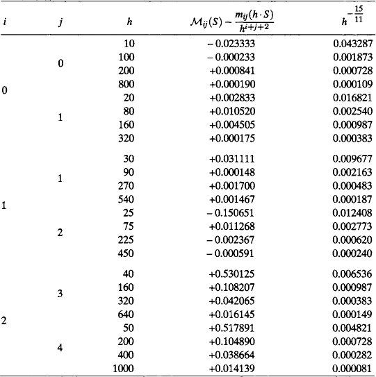
TABLE 17.5
Errors in approximating Mij(S) by h−(i + j + 2) · mi,j(h · S) for different grid resolutions h, where S is the bounded region whose frontier consists of four segments of the quartic curve (y − 5)2 =(4(x − 2)2 − 4)2.

| M00(S) = 10.66667 | M01(S) = 53.33333 |
| M11(S) = 106.6667 | M12(S) = 611.3523 |
| M23(S) = 8005.587 | M24(S) = 53289.62 |
The values in both tables are given for the same values of h to illustrate two things:
1) The effect of the sizes of the real moments that are to be estimated: As can be seen from Table 17.5, if these moments have relatively large values, the required precision is not achieved for small values of h as it was in the previous examples; higher resolutions h have to be used. It is more appropriate to use the relative error in such situations. If we use the usual definition of relative error and Theorem 17.4 is applied to regions that have no straight segments on their frontiers, then we have the following:
2) The effect of the elongation of the region: For example, m = 5 gives a greater elongation than m = 2. No theoretic results on this subject have yet been obtained, but it seems that an increase in elongation leads to an increase in worst-case error.
It might also be of interest to calculate errors in moment estimates for values of m such that both m and h go to infinity (e.g., m = log h, ![]() , m = h2).
, m = h2).
17.4 Operations on Pictures and Invariant Properties
Let P be the set of pictures P defined on a given grid, and let Φ be a function from P into itself. Φ is called a pixel−wise operation (or a “point operation ”) if the value of (Φ(P))(p) depends only on the value of P (p). It is called a local operation if the value of (Φ(P))(p) depends only on the values of a set of P(q)s such that p is one of the qs and maxq(de(p, q)) is constant so that it does not depend on the size of the picture. It is called a geometric operation if there exists a function g from the grid into itself such that the value of (Φ(P))(p) depends only on the values of a set of P(q)s such that maxq((g(p),q)) is constant and so does not depend on the size of the picture. Pixelwise and local operations are studied in books about digital picture processing. For more about geometric operations see Chapter 14.
A picture property ![]() is called invariant under Φ if
is called invariant under Φ if ![]() (Φ(P)) = F(P) for all P ∈ P. For example, let Φ be the linear pixel-wise operation that takes P(p) into aP (p) + b. A ratio of differences of pixel values (e.g.,
(Φ(P)) = F(P) for all P ∈ P. For example, let Φ be the linear pixel-wise operation that takes P(p) into aP (p) + b. A ratio of differences of pixel values (e.g., ![]() ), is invariant under Φ, because the following is true:
), is invariant under Φ, because the following is true:
The set of values of the pixels of P is invariant under any one-to-one mapping of P into itself; in particular, it is invariant under any one-to-one geometric transformation of P (see Section 14.4). It follows that any ![]() (P) that depends only on the set of values of P (e.g., any statistic property such as m00) is invariant under any one-to-one Φ. Evidently, m20(P) is invariant under reflection of P in the y-axis; this is similar for m02(P) and the x-axis; and m0(P) is invariant under reflection of P in the origin or under any one-to-one rotation of P around the origin.
(P) that depends only on the set of values of P (e.g., any statistic property such as m00) is invariant under any one-to-one Φ. Evidently, m20(P) is invariant under reflection of P in the y-axis; this is similar for m02(P) and the x-axis; and m0(P) is invariant under reflection of P in the origin or under any one-to-one rotation of P around the origin.
Properties that are invariant under various types of (real) geometric transformations are studied in various branches of geometry (see Section 14.1); however, because most geometric transformations do not take pictures into pictures (see Section 14.5), properties that are invariant under real geometric transformations are at best “approximately invariant ” when the transformations are applied to pictures.
17.5 Spatial Relations
Properties of binary pictures can be regarded as properties of the sets of 1s in the pictures (e.g., as properties of [not necessarily connected] “objects ”). Relative values of properties of pictures define relations between pictures, and this is similar for relations between objects. In this section, we briefly discuss two types of “spatial ” (i.e., geometric) relations between objects: relations of relative position and topologic relations.
17.5.1 Relations of relative position
Quantitative relations of relative position between single pixels can be defined by fuzzy subsets of the grid. For example, if p = (x,y), the degree of membership of q = (u,v) in “above p ” can be defined by a fuzzy subset μa(ρ) such that μa(p)(x,v) = 1 for all v> y;μa(ρ)(u,v) decreases monotonically as |u – x| increases; and μa(ρ)(u,v) = 0 for v < y. Similarly, “near p ” can be defined by a fuzzy subset μn(ρ) such that μa(P)(x,y) = 1 and μn(ρ)(u,v) decreases monotonically as d((u,v), (x,y)) increases.
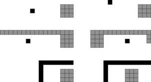
It is much harder to define relations of relative position between sets of pixels. To see this, consider Figure 17.8, which illustrates the difficulty of defining “to the left of.” Let A be the black object and B the gray object. If we require that every pixel of A be to the left of every pixel of B, we exclude all but the two upper cases; however, excluding the lower left case seems unreasonable. If we require only that every pixel of A be to the left of some pixel of B, we include all but the case on the lower right; however, including the case on the middle right seems unreasonable. If we require that A ’s centroid be to the left of B’s centroid, we include all but the case on the middle right; however, including the case on the lower right seems unreasonable. One proposed definition requires that two conditions be satisfied: A ’s centroid must be to the left of B′s leftmost pixel and A′s rightmost pixel must be to the left of B′s rightmost pixel. This definition excludes the two middle cases and the lower right case, which is defensible. Another possibility is to require that every pixel of A be to the left of some pixel of B and every pixel of B be to the right of some pixel of A. This excludes all but the two upper cases; it includes the lower left case if the rightmost pixel of A is removed. Note that this definition implies that the “to the left of ” relation is transitive, and its inverse is “to the right of.” The relation would also be reflexive if we required that every pixel of A be to the left of or in the same column as some pixel of B and that every pixel of B be to the right of or in the same column as some pixel of A. However, a purely coordinate-based definition of this type may not be adequate in all cases; judgments about “to the left of ” can be influenced by the interpretation of the picture as a projection of a 3D scene or by the recognition of A and B as familiar objects.
17.5.2 Topologic relations
We recall that any adjacency relation on a grid defines an adjacency relation between disjoint subsets of the grid: S and T are called α−adjacent iff some pixel of S is α-adjacent to some pixel of T. For any such adjacency relation, we can also define quantitative measures of degree of adjacency (e.g., in terms of what fraction of the pixels of S are adjacent to pixels of T or vice versa); see Exercise 5.
We have also seen that an adjacency relation defines separation relations between disjoint subsets of the grid. Let U, V, and W be sets of pixels such that U and V are disjoint. We say that W α−separates U from V iff any α-path from a pixel of U to a pixel of V must contain a pixel of W. More generally, let μ, v, and ω be fuzzy subsets of a picture. We say that ω α-separates μ from v iff, on any α-path ρ = (p0,…,pn), there exists a pixel pi(1 ≤ i < n) such that ω(pi) ≥ max(μ(p0),v(pn)).
Surroundedness is a special case of separateness; in a binary picture, we say that S surrounds U if it separates U from the infinite background component B of the picture. Quantitative measures of degree of surroundedness can also be defined. For example, let U = {p}, and let W not contain p. The following are two ways of measuring the degree to which W surrounds p in a 2D picture:
a) Evidently, W separates U from B if it separates U from the border ϑB of B, which is finite; let ϑB consist of n pixels. For each b ∈ ϑB, let ![]() be a digital straight line segment with endpixels p and b. If m of the n
be a digital straight line segment with endpixels p and b. If m of the n ![]() intersect W, we say that the degree of v−surroundedness (“visibility surroundedness ”) of p by W is m/n.
intersect W, we say that the degree of v−surroundedness (“visibility surroundedness ”) of p by W is m/n.
b) We define the degree of τ-surroundedness (“turn surroundedness ”) of p by W as min(τ (ρ)), where τ (ρ) is the total turn of ρ (see Chapter 10, Exercise 6) and the min is taken over all 4-paths ρ from p to ϑB that do not intersect W. If no such ρ exists (i.e., if W 4-surrounds {p}), we say that the degree of τ-surroundedness of p by W is infinite.
In a 3D picture under (α,α′)-adjacency, if the Euler characteristic of a set W is equal to the number of α-components of W minus the number of α′-components of ![]() , W is called tunnel−free. Let W and Z be α-connected sets, each of which is contained in the background component of the other (so they are disjoint). It can be shown that W is tunnel-free iff Z is tunnel-free. Let W* be a tunnel-free set that contains W. We say that W and Z are linked if any such W* intersects Z. It can be shown that this implies that W and Z are not tunnel-free.
, W is called tunnel−free. Let W and Z be α-connected sets, each of which is contained in the background component of the other (so they are disjoint). It can be shown that W is tunnel-free iff Z is tunnel-free. Let W* be a tunnel-free set that contains W. We say that W and Z are linked if any such W* intersects Z. It can be shown that this implies that W and Z are not tunnel-free.
A (simple) 3D curve can be knotted, and a set of pairwise disjoint 3D curves can be linked [768]. A curve can therefore be called a knot, and a finite union of pairwise disjoint curves can be called a link. A knot or link is called polygonal if the curves are (real) polygons, and it is called digital if they are isothetic grid polygons. Two knots or links are called (knot-theoretically) isomorphic iff there exists an orientation-preserving homeomorphism that maps one of them onto the other. A knot is called unknotted if it is isomorphic to a simple planar polygonal curve.
Two simple polygons Q and Q′ are said to differ by an elementary deformation if there exist three points p, q, and r such that Q intersects the planar triangular region pqr in the line segment pr; Q′ intersects pqr in the line segments pq and qr; and Q and Q′ are otherwise identical. It can be shown that two polygonal knots or links are isomorphic iff they differ by a finite sequence of elementary deformations. A similar definition can be given for digital knots or links using deformations that take three sides of a rectangle into the fourth side. (Note that this is not the same as the elementary deformations of digital curves in Section 16.4.)
The parallel projection Lθ of a polygonal link L in direction θ (onto a plane perpendicular to θ) is the union of a connected set of straight line segments. We call Lθ regular if the following are true:
a) For all but finitely many points p of Lθ, the preimage of p is a single point of L.
b) Each of the exceptional points has a preimage that is an interior point of exactly two polygon sides of L.
It is not hard to see that, for any polygonal link L, there exist directions θ for which Lθ is regular. An exceptional point p in a regular projection of L is called a crossing point. The two preimages of p on L have different coordinates with respect to a coordinate axis in direction θ. These two preimages lie on two polygon sides of L; the side with a preimage that has a higher (lower) coordinate is said to cross over (under) the other side. It is easy to show that, if some regular projection of a knot K never crosses itself, K must be unknotted.
If, in some regular projection of a link L, some knot K crosses only over or under the other knots (or does not cross them at all), K cannot be linked to the other knots. It can be shown that W is not tunnel-free iff there exist a simple α-curve K contained in W and a simple α′-curve K′ contained in W such that K and K′ are linked.
17.6 Exercises
1. Let P1,…,Pn be distinct pictures defined on a given grid. Prove that there exist pixels p1,…,pn−1 such that, for any 1 ≤ i ≠ j ≤ n, we cannot have Pi(p1) = Pj (p1),…,Pi(pn−1)=Pj (pn−1).
2. Let P be a binary picture defined on an k-pixel grid. Let ![]() be a predicate on this class of pictures, and let Φ be a Boolean function of k variables such that
be a predicate on this class of pictures, and let Φ be a Boolean function of k variables such that ![]() (P) is true iff Φ(P) = 1; such a Φ is called a Boolean expression for
(P) is true iff Φ(P) = 1; such a Φ is called a Boolean expression for ![]() . The length of the shortest Boolean expression for
. The length of the shortest Boolean expression for ![]() is called the length of
is called the length of ![]() . Let
. Let ![]() 1(
1(![]() 1 +) be the predicate that is true iff exactly (at least) one pixel of P has value 1. Prove that the length of
1 +) be the predicate that is true iff exactly (at least) one pixel of P has value 1. Prove that the length of ![]() is k and that the length of
is k and that the length of ![]() 1 cannot be a linear function of k but is at most k2.
1 cannot be a linear function of k but is at most k2.
3. Prove that, if P is symmetric around the line y = x (i.e., f(x, y) = f(y, x) for all x, y), then mij(P) = mji(P) for all i,j.
4. Prove that the principal axis is in the direction of the eigenvector of the following matrix, which corresponds to its larger eigenvalue:
5. Let S be a nonempty finite 4-connected subset of Z2, and let T be a subset of Z2 that is disjoint from S. Let ∂TS be the set of pixels of S that are 4-adjacent to pixels of T; note that, if ![]() is the border of S. Define the degree of adjacency of S to T as follows:
is the border of S. Define the degree of adjacency of S to T as follows:
Evidently, 0 ≤ aT (S) ≤ 1. For what proper subsets T of Z2 do we have aT (S) = 1? If T is nonempty, finite, and 4-connected, how is aS(T) related to aT(S)?
17.7 Commented Bibliography
Properties for which the cardinality or the diameter of σ does not depend on the picture size are studied in [733] and [533, 534].
Exercise 1 is based on [360] and Exercise 2 on [439]. Theorem 17.1 was first applied to digital pictures in [880].
Moments were introduced into picture analysis in [446]; see also [362] and [15]. For elongatedness Θ(S), see [468, 1113]. (For an “intrinsic ” definition of elongatedness, see Section 15.6.2.) For the approximation of real moments by digital moments, see [558, 559], [560], [1113]. [561] gives the upper bound example that follows Theorem 17.2. Section 17.3 reviews [562]. For other types of moments, see [980].
For invariants in geometry, see [559, 560]. For the difficulty of defining “to the left of,” see [1127]. For measures of degree of adjacency or surroundedness, see [913]. For digital knots and links, see [338, 768].
1See also Definition 8.7.
2This was independently discovered by both M. Fr échet and F. Riesz; see [855].