
Curves and Surfaces: Topology
On the basis of the concepts introduced in Chapter 6, this chapter discusses curves and surfaces in topologic spaces, with emphasis on the digital case.
7.1 Curves in the Euclidean Topology
The definition of a curve has an interesting history in mathematics. Jordan curves are defined by parameterization; see the “parameterized paths ” in Section 6.3.3. Urysohn-Menger curves are defined using a topologic approach. The two definitions are equivalent, and they both define separations of the plane.
7.1.1 Jordan curves
Let φ be a parameterized continuous path φ :[a, b] → R2 such that a ≠ b, φ (a) = φ(b), and let φ(S) ≠φ(i) for all s,t (a ≤ s<t<b). The following set was defined by C. Jordan in 1893 to be a Jordan curve in the plane1:
Similarly, a Jordan arc γ in the plane is defined by a subinterval [c, d] where a ≤ c < d ≤ b. A Jordan curve is topologically equivalent (homeomorphic) to a unit circle; it does not have “crossings ” or “touchings.” A rectifiable Jordan arc γ has a bounded arc length as follows, where de is the Euclidean metric:
C. Jordan proposed, in 1883, a definition of a parameterized curve in the following form:
Using a parameterization that satisfied Equation 7.3, G. Peano defined, in 1890, a curve known as the Peano curve that fills the whole unit square. (One iteration of the construction of the Peano curve is shown in Figure 1.7.) Note that Equation 7.1 excludes the Peano curve. However, Equation 7.3 is still in common use for arc length calculation. (Evidently, Equation 7.3 follows from Equation 7.1;α and β can be defined by projecting φ on the x- and y-axis, respectively. However, Equation 7.3 allows for (x,y) ∈γ such that x = α(t1) and y = β(ttesub2), with t1 ≠ t2.) If α and β are differentiable functions, the arc is called differentiable, and its arc length is as follows:
The Jordan definition applies to curves that have parametric forms. Not all curves have such forms, and, even if they do, the forms may be difficult to find. (See Chapter 8 about the geometry of Jordan curves.) In picture analysis, we have to deal with curves that are given in digitized pictorial form and for which a parametric description is often not of interest. Topologic methods of defining curves are therefore more relevant for our purposes.
7.1.2 Urysohn-Menger curves
The local (adjacency-based) approaches used for curve tracing in picture analysis are related to nonparametric curve characterizations based on topologic connectedness.
Let [S, d] be a metric space. p ∈ S is called a point of accumulation of M ⊆ S iff, for any ε > 0, the ε-neighborhood Uε(p) of p contains a point q ≠ p of M. It can be shown that M is topologically connected in S iff, for any partition of M into two disjoint subsets, some point in one of the subsets is a point of accumulation of the other subset.
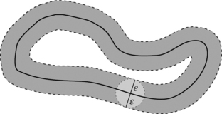
G. Cantor was the first to suggest a topologic definition of a curve, but his definition had to be revised. P. Urysohn provided a correct definition in 1923, and K. Menger did so independently in 1932. Let M ⊆ L ⊆ Rn. p ∈ Rn is called an L-frontier point of M iff, for any ε > 0, the ε-neighborhood Uε(p) of p contains points of M as well as points of L/M. The set of L-frontier points of M is called the L-frontier of M. A continuum M ⊆ Rn is called one-dimensional at p ∈ M iff, for some ε> 0, any continuum C contained in the M-frontier of Uε(p) n M is a singleton {q}; see Figure 7.1. M is called one-dimensional iff it is one-dimensional at every p ∈ M. Note that this allows “one-dimensional ” to be defined in a non-Aleksandrov space. (In an Aleksandrov space, we can use Definition 6.7.)

This definition was originally given only for the Euclidean topology. Note that an isolated point in Rn satisfies this definition.
A Urysohn-Menger curve is more general than a Jordan curve; it may be a simple curve see (Definition 7.3) that forms a loop without any self-intersections, but it may also be a union of finitely many bounded arcs.
Dimension theory, as established by P. Urysohn and K. Menger, is based on a generalization of the definition of one-dimensionality at p given above. A metric space (or manifold) S has dimension n at p ∈ S if S can be disconnected by removing an arbitrarily small set of dimension n −1 that contains p but not by removing a set of smaller dimension. We will return to this approach when we discuss surfaces (2D manifolds).
Let γ ⊂ E2 be a Jordan curve, and let ε> 0. The ε-tube of γ is the set of all points p such that de({p},γ) ≤ε, where de is Hausdorff distance. The frontier of any ε-tube of a Jordan curve that is topologically equivalent to an annulus (see Figure 7.2) consists of two disjoint Jordan curves, and the de Hausdorff distance between these curves is 2ε.
P.S. Aleksandrov proved that Urysohn-Menger curves can be approximated by polygonal chains:
Thus a Urysohn-Menger curve γ is in the ε-tube of a polygonal chain for arbitrarily small ε> 0.
7.1.3 Simple curves and arcs
A curve γ has branching index m ≥ 0 at p ∈γ iff, for any r> 0, there is a positive real ε<r such that the cardinality of the γ-frontier of Uε(p) ∩γ is at most m. For a sufficiently small real r> 0, it follows that, for any positive real ε<r, the cardinality of the γ-frontier of Uε (p)∩γ is at least m. Note that the definition of a curve allows m to be countably infinite.
A basic theorem in the mathematic theory of curves is as follows:
This theorem shows that Theorem 7.1 also applies to Jordan curves.
A regular point of a curve has branching index 2 and is not an endpoint. A branch point has branching index 3 or greater. A singular point is either an endpoint or a branch point. The topologic concept of branching index is relevant to the study of skeletons (see Chapter 16).
7.1.4 Elementary curves and the Euler characteristic
An elementary curve is the union of a finite number of simple arcs, each pair of which have at most a finite number of points in common. It consists of a finite number of singular points and a finite number of regular components; the latter are either simple curves or simple arcs. Every regular point p ∈ γ is on a uniquely determined subcurve γρ ⊆ γ that is either a simple curve (the component of p in γ), a simple arc that has only one endpoint, or a simple arc that has two endpoints.
If we partition a simple curve γ (e.g., by choosing two points of γ [αtesub0 = 2] that divide γ into two simple arcs [α1 = 2]), we find that the Euler characteristic χ(γ) is α0 –α1 = 0. An elementary curve with at least one singular point on each of its simple curves is a one-dimensional Euclidean complex. The Euler characteristic of such a complex is equal to the number of singular points minus the number of regular components. For example, a simple arc that has only one endpoint, which is also a complex of a simple curve, has Euler characteristic 0.
Figure 7.3 (left) shows an elementary curve that is a union of simple arcs. Figure 7.4 shows the capital letters of the German alphabet; the letters are assumed to be elementary curves. (Note that a rectangle of nonzero width [e.g., a thick line segment] is not homeomorphic to a line segment.) The three (pairwise nonhomeomorphic) letters Ä, Ö, and Ü have three components each as compared with only one component for each of the remaining letters; hence these three letters cannot be homeomorphic to any of the other letters.

FIGURE 7.3 Left: an elementary curve with Euler characteristic 9 − 10 = −1; it has nine singular points and 10 regular components. Right: two partitions of the curve into one-dimensional geometric complexes, both with Euler characteristic 12 − 13 = −1.

FIGURE 7.4 Capital letters of the German alphabet. We assume that the letters are elementary curves that may have endpoints or branch points, as indicated on the right for the letters A and B.
The homeomorphy of the letters in Figure 7.4 depends on whether we consider a letter to be a set that is not one-dimensional at any of its points or to be an elementary curve. Figure 7.5 shows both alternatives for two letters. The elementary curve version of the letter E has a decomposition vertex (i.e., deletion of this point partitions the set into more than two connected parts), but the elementary curve version of the letter M has no decomposition vertex. The number of decomposition vertices is a topologic invariant (i.e., it is preserved by homeomorphism).

FIGURE 7.5 The two sets on the left are homeomorphic, but the two elementary curves on the right (which are not linear skeletons of the sets on the left, although they may be regarded as “skeletons ” in a picture-analysis context) are not.
As an illustration of isotopy, consider the sets of curves 05 and 20. These sets are isotopic to each other but not to the set 97, because 9 is not homeomorphic to 0.
7.1.5 Separation theorems
The Jordan-Veblen curve theorem of Euclidean topology says that any set that is topologically equivalent to a unit circle decomposes the Euclidean plane into two disjoint sets.
This theorem was first stated by C. Jordan in 1887. His proof (which was incorrect) attempted to use a sequence of polygons that converged to the curve.2 The first correct proof was given by O. Veblen in 1905 using the parametric characterization of the curve. This proof left open the question of whether the inside and outside of the curve are always topologically equivalent to the inside and outside of a circle. The stronger Schönflies-Brouwer curve theorem is as follows:
The proof by A. Schönflies in 1906 contained some errors, which were fixed by L.E.J. Brouwer in 1910. Both theorems also apply to simple Urysohn-Menger curves (see %Theorem 7.2). By the Schönflies-Brouwer theorem, any two simple curves in E2 are isotopic; this is a stronger result than the Jordan-Veblen theorem.
7.2 Curves in Incidence Grids
The Urysohn-Menger method of defining curves see (Definition 7.2) can be adapted to the grid cell topologies [Cn, ≤]. We make use of the dimension dimA defined by adjacency relation A; see Definition 6.7. This definition applies to arbitrary subsets of incidence grids (e.g., subsets that define frontiers and do not contain principal nodes).
7.2.1 Frontier grids; curves of marginal nodes
Section 5.4.3 defined a frontier grid for a 2D picture. Such grids can also be defined for 3D (or even nD) pictures; they were proposed and used (with different terminology and notation) for 2D and 3D picture analysis by V. Kovalevsky [594].
Equation 5.3 guarantees the existence of such an isomorphism.
Figure 7.6 illustrates frontiers in a 2D incidence grid (left) and their representations in the 2D frontier grid using a 2D incidence grid model representation (middle) and a (simpler) 4-adjacency grid model representation (right).

FIGURE 7.6 Left: two frontiers in the 2D incidence grid. Middle: representations of these frontiers in an incidence grid model of the frontier grid. Right: their representations in a 4-adjacency grid model of the frontier grid.
Proof The frontier contains only 0- and 1-cells. A 0-cell is incident with up to four 1-cells, and each 1-cell is incident with two 0-cells. These are one-dimensional configurations; see Definition 6.7. The frontier is closed, because it always contains the two 0-cells that are incident with each of its 1-cells, and it is bounded because the region is finite.
This proposition shows that the frontiers of regions in the 2D incidence grid are curves in the sense of Definition 7.2. The definition of branching points also applies, so that simple curves, simple arcs, and elementary curves can be defined. The curves are 4-curves in the 4-adjacency representation of the frontier grid. The 4-curves that represent the frontiers of two regions in the picture can be 4-adjacent in the frontier grid; see Figure 7.6.
7.2.2 Curves of principal nodes
We are particularly interested in one-dimensional connected sets of pixels or voxels in the picture grid; see the middle of Figure 6.11. In this section, we describe a way of defining curves in an incidence grid without making use of the frontier grid.
We recall that a region M is a complete finite component of Cn and that its core is a nonempty maximal connected set of principal nodes; see Section 5.1.3. A closed region in C2 is 2D when we use the definition of dimension based on adjacency (Definition 5.3); hence we cannot use closed regions to model curves. Rather, we define a curve ρ of principal nodes as a one-dimensional region in [Cn, ≤] (n ≥ 2). It follows that any curve has finite cardinality, so the union ![]() ρ of the cells of ρ is bounded.
ρ of the cells of ρ is bounded. ![]() ρ is an isothetic polygon if ρ is a curve in C2 and an isothetic polyhedron if ρ is a curve in C3.
ρ is an isothetic polygon if ρ is a curve in C2 and an isothetic polyhedron if ρ is a curve in C3.
Figure 7.7 illustrates this definition. The upper row shows curves in which the connectedness between principal cells is based on 1-connectedness; they are therefore called 1-curves. Note that the example in the upper left corner also contains 0-cells, but it is still one-dimensional, and these 0-cells add no further connectivities to the curve. From now on, we exclude 0-cells from 1-curves; see the definition of minimal curves below. Pixels (2-cells) in a 1-curve can “touch ” (i.e., they can be 0-adjacent); see the examples in the middle and on the right in the upper row of Figure 7.7.

FIGURE 7.7 Upper row: 1-curves; the curve on the left is a 1-curve after removing three 0-cells. Middle row: 0-curves. Bottom row, upper part: sets that are not curves; lower part: see text.
The middle row of Figure 7.7 shows curves in which connectedness between principal nodes is based on either 1-adjacency or 0-adjacency (in the sense of Definition 5.2). Such curves are called 0-curves. The example in the middle forms an “8”.
The upper examples in the bottom row of Figure 7.7 are not curves. The examples on the left and in the middle are not regions, because they are not complete, and the example on the right is not one-dimensional. (The three examples in the lower positions will be explained later in this section.)
An α-curve ρ is called minimal iff it contains only marginal cells that are required for its connectivity. For example, in the upper left of Figure 7.7, we obtain a minimal 1-curve after removing three 0-cells and one “terminal ” 1-cell. (Note that removal of a 1-cell instead of a 0-cell may preserve connectivity between principal cells but will result in a noncomplete set.) It follows that an α-curve ρ is minimal iff it contain only i-cells (α ≤ i ≤ n −1) that are i-adjacent to two principal nodes in the core of ρ. For example, in the upper right of Figure 7.7, we obtain a minimal 1-curve after removing two “terminal ” 1-cells. It follows that a minimal (n −1)-curve in Cn is always an open region. (Note that a 0-curve cannot be closed, because it is one-dimensional.)
A vertex of a 0-cell in a 0-curve ρ is called a decomposition vertex if its deletion partitions ![]() ρ into more than two connected components in the Euclidean topology. Minimal 1-curves do not have decomposition vertices.
ρ into more than two connected components in the Euclidean topology. Minimal 1-curves do not have decomposition vertices.
An α-curve ρ is called confirmative iff, for any two principal nodes in ρ that are adjacent via some i-cell (α ≤ i ≤ n), there is also a marginal cell in ρ that ensures this adjacency, and adding this cell does not contradict one-dimensionality. For example, the 0-curve on the lower left in Figure 7.7 is not confirmative, but adding one 0-cell makes it confirmative, and it remains one-dimensional. Note that completeness of curves does not imply confirmativeness. The 1-curves in the middle and right of the upper row in Figure 7.7 are confirmative, because 0 <α = 1. The 0-curve at the center of Figure 7.7 is confirmative, but adding the related 0-cell would destroy its one-dimensionality. From now on, we will assume that α-curves in the incidence grid are minimal and confirmative.
A curve ρ has branching index m ≥ 0 at a principal node p iff exactly m principal nodes q ∈ ρ are adjacent to p. For n = 2 (0- or 1-curves), possible branching indices are 1 (an endnode), 2 (a regular node), and 3 or 4 (a branch node). For n = 3 (0-, 1- or 2-curves), a branch node can have branching indices 3, 4, 5, or 6. A node is called singular if it is either an endnode or a branch node.
Elementary curves differ from curves, because some of their principal nodes can be explicitly labeled as being endnodes of arcs. A simple curve (arc) has a circuit (sequence) of principal nodes. The number of principal nodes in the circuit (sequence) defines the length of the curve (arc). The bottom row of Figure 7.7 shows that the shortest simple 1-curve in C2 has length 8 and that the shortest simple 0-curve in C2 has length 4.
Proposition 7.2
A curve ρ in [C2, ≤] is a simple 1-curve iff ![]() ρ is homeomorphic to an annulus; it is a simple 0-curve iff
ρ is homeomorphic to an annulus; it is a simple 0-curve iff ![]() ρ is homotopic to a circle.
ρ is homotopic to a circle.
The union of the cells in an elementary plane curve ρ is a (not necessarily connected) isothetic polygon ![]() ρ that has a frontier γ = ϑ (
ρ that has a frontier γ = ϑ (![]() ρ) that is an elementary isothetic curve. If ρ is a simple 1-curve, this frontier splits into two nonempty simple curves γ1 and γ2. We recall that ° denotes the topologic interior (see Section 3.1.7). Let θ0 be the side length of the large squares in the geometric representation of C2 (θ0 is “slightly smaller ” than the grid constant θ in our topologic representation and is equal to θ in the original grid cell representation).
ρ) that is an elementary isothetic curve. If ρ is a simple 1-curve, this frontier splits into two nonempty simple curves γ1 and γ2. We recall that ° denotes the topologic interior (see Section 3.1.7). Let θ0 be the side length of the large squares in the geometric representation of C2 (θ0 is “slightly smaller ” than the grid constant θ in our topologic representation and is equal to θ in the original grid cell representation).
7.3 Curves in Adjacency Grids
A curve can be regarded as a sequence of pixels or voxels in an adjacency grid (in either the grid point or grid cell model). Figure 7.8 shows examples of simple (n − 1) -curves and (n – hbox 1) -arcs in 2D and 3D. Note that this simple representation does not uniquely characterize the curve. For example, the 2D object on the left in Figure 7.9 may be either a simple 8-curve or a nonsimple 0-curve, and this is the same for the 3D object on the right. Note that, in the incidence grid, the ambiguities in these figures can be removed by deleting a marginal cell (the 0-cell at which the object “touches itself ”).

FIGURE 7.8 Simple (n − 1)-curves (left) and simple (n − 1)-arcs (right) for n = 2 in the upper row and n = 3 in the lower row.

FIGURE 7.9 Left: the 2D object is either a simple 1-curve or a nonsimple 0-curve. Right: a similar case in 3D.
7.3.1 Euler characteristics of curves
The Euler characteristic of a simple curve in the Euclidean plane is 0; see Section 7.1.4. The Euler characteristic of a simple 0- or 1-curve can be calculated by considering the curve in the incidence grid (see Definition 5.14) as a 2D Euclidean complex. In general, the Euler characteristic of a region M is calculated by decomposing RM into a Euclidean complex and applying Definition 5.14. For example, the simple 1-curve ρ shown on the upper left in Figure 7.8 has α0 = 64 grid vertices,α1 = 96 grid edges, and α2 = 32 grid squares so that its Euler characteristic is χ = α0 –α1 +α2 = 0.
The dual interpretation of a set of 2-cells in the grid point model leads in general to a 2D Euclidean complex. In our 1-curve example, however, we obtain only a one-dimensional Euclidean complex that has α0 = 32 0-cells (centers of grid squares) connected by α1 = 32 1-cells, so we get the following:
The interpretation of ρ in the grid point model can also be regarded as a planar-oriented adjacency subgraph G of Z2. G has α0 = 32,α1 = 32, and α2 = 2; there are no atomic cycles in this example, but we must count one inner and one outer border cycle. However, the Euler characteristic of G is not the quantity we are interested in for characterizing ρ. For our 1-curve example, we have the following:
The Euler characteristic χ + of a planar-oriented adjacency graph is always 2 (see Theorem 4.6). The curve ρ can also be interpreted as a 2-strong planar-oriented adjacency subgraph in the frontier grid (see Section 5.4.3) of grid vertices, with 32 atomic cycles and two border cycles (i.e.,α2 = 34) and with α0 = 64 and α1 = 96, which also leads to χ + = 2. This is a graph-theoretic characterization only; it does not make distinctions between faces.
7.3.2 Simple 2D curves
In 2D, we have t4 = 4 and t8 = 3. In fact, a simple 4-curve must have a length of at least 8.
A pixel p = (i,j) is inside a simple 4-curve ρ iff p is not on ρ and the grid lines i and j cross ρ an odd number of times on each side of p. For an illustration of this property in the grid point model, see Figure 7.10 (left). Evidently, the grid line crosses the curve to the left of p. On the right of p, the grid line only “touches ” the curve, because it “comes in from ” and “goes out to ” the same halfplane; however, further to the right, it crosses the curve, because it “comes in from ” and “goes out to ” different halfplanes. (We will not give a formal definition.) p is outside ρ if it is neither on nor inside ρ. The inside and outside of a simple 8-curve are defined analogously. Note that the set of pixels inside a simple 4-curve may not be 4-connected; see Figure 7.10 (left).

FIGURE 7.10 Left: a pixel p inside a simple 4-curve. Right: a simple 4-curve for which decisions about inside and outside are more difficult (e.g., is q inside or outside?).
Let G(ρ) be the set of all pixels on a path ρ.3 Two 4- or 8-paths ρ1 and ρ2 intersect iff G(ρ1) ∩ G(ρ2) ≠ø. Figure 7.11 shows that two 8-paths can “cross ” without intersecting. Let p and q be the pixels that are not in the set S. We say that S 8-separates (4-separates) p and q iff any 8-path (4-path) from p to q intersects S. In particular, this definition can be applied to the set S = G(p) of pixels on a path ρ.

Theorem 7.6
A simple 4-curve (8-curve)ρ 8-separates (4-separates) all pixels inside ρ from all pixels outside ρ.
Proof We prove the theorem for simple 4-curves and 8-separation; the case of simple 8-curves and 4-separation can be treated analogously. For simplicity, in this proof we identify an (ordered) path ρ with its (unordered) pixel set G(p), and we denote the complement of G(p) with ![]() .
.
We first prove that, for any simple 4-curve ρ, there is at least one pixel inside and at least one pixel outside ρ. Because ρ is finite, there are infinitely many pixels outside ρ. To see that the inside of 8 is nonempty, let pm = (x, y) be the uppermost of the rightmost pixels on ρ; then (x − 1, y) and (x, y −1) must both be on ρ, because they are the only possibilities for pm−1 and pm+1. If (x – 1,y −1) were on ρ, according to (C3)in Definition 7.7, it would have to be both pm−2 and pm+2 so that by (C2) we would have m − 2 = m + 2 (modulo n + 1), which is impossible, because n ≥ 4; hence (x − 1, y−1) is in ![]() . It follows that (x, y − 2) is on ρ. Indeed, if (x – 1,y) is pm−1, it is the only possibility for pm−2, whereas, if (x − 1, y) is pm+1, it must be pm+2. Let Hp = {(x + i,y): i ∈ N} be the horizontal digital ray that emanates from pixel p = (x,y) to the right. We have just proved that H(x-1,y-1) crosses ρ exactly once, namely at (x,y −1); hence (x − 1, y−1) is inside ρ. Let p0 be inside ρ and pm outside ρ. Let φ = (p0, p1,…, pm) be an 8-path, and suppose that every pj is in
. It follows that (x, y − 2) is on ρ. Indeed, if (x – 1,y) is pm−1, it is the only possibility for pm−2, whereas, if (x − 1, y) is pm+1, it must be pm+2. Let Hp = {(x + i,y): i ∈ N} be the horizontal digital ray that emanates from pixel p = (x,y) to the right. We have just proved that H(x-1,y-1) crosses ρ exactly once, namely at (x,y −1); hence (x − 1, y−1) is inside ρ. Let p0 be inside ρ and pm outside ρ. Let φ = (p0, p1,…, pm) be an 8-path, and suppose that every pj is in ![]() . Because p0 is inside ρ and pm is outside ρ, there must exist some i (0 < i ≤ m) such that pi1 is inside and pi is outside. If pi1 and pi are horizontally adjacent, this is impossible by definition of “inside ” and “outside ”. On the other hand, if they are vertically or diagonally adjacent, Hi-1 and Hi (where we have omitted the ps for brevity) are vertically adjacent rays. Let R = [qk+1,…, qk+r} be a run (maximal consecutive sequence) of pixels in which ρ intersects Hi-1 R Hi; thus each of qk and qk+r+1 is either above or below both Hs. (Because pi −1 and pi are 8-adjacent, a run of 4-neighbors cannot leave Hi-1 R Hi but rather remain on the union of the rows that contain them; the run can leave only by passing to the row above or below.) Suppose they are both above; if they are both below, we can use exactly analogous arguments. We can assume, without loss of generality, that Hi−1 is the upper of the two Hs. If all of qk+v…, qk+r are on Hi-1, then ρ touches Hi-1 in R and does not even touch Hi in R, so it crosses neither of the Hs in any subset of R. On the other hand, if some of these qs are on Hi, let qs be the first one and qt the last one. Then Hi-1 crosses ρ in [qk+v…, qs-1} and Hi crosses it in [qv+v…, qk+l}, but neither of them can cross it anywhere between qu and qv by the same argument as given in the preceding paragraph. Thus, in this case, both Hi-1 and Hi cross ρ just once in subsets of R.
. Because p0 is inside ρ and pm is outside ρ, there must exist some i (0 < i ≤ m) such that pi1 is inside and pi is outside. If pi1 and pi are horizontally adjacent, this is impossible by definition of “inside ” and “outside ”. On the other hand, if they are vertically or diagonally adjacent, Hi-1 and Hi (where we have omitted the ps for brevity) are vertically adjacent rays. Let R = [qk+1,…, qk+r} be a run (maximal consecutive sequence) of pixels in which ρ intersects Hi-1 R Hi; thus each of qk and qk+r+1 is either above or below both Hs. (Because pi −1 and pi are 8-adjacent, a run of 4-neighbors cannot leave Hi-1 R Hi but rather remain on the union of the rows that contain them; the run can leave only by passing to the row above or below.) Suppose they are both above; if they are both below, we can use exactly analogous arguments. We can assume, without loss of generality, that Hi−1 is the upper of the two Hs. If all of qk+v…, qk+r are on Hi-1, then ρ touches Hi-1 in R and does not even touch Hi in R, so it crosses neither of the Hs in any subset of R. On the other hand, if some of these qs are on Hi, let qs be the first one and qt the last one. Then Hi-1 crosses ρ in [qk+v…, qs-1} and Hi crosses it in [qv+v…, qk+l}, but neither of them can cross it anywhere between qu and qv by the same argument as given in the preceding paragraph. Thus, in this case, both Hi-1 and Hi cross ρ just once in subsets of R.
We have thus shown that, in any case, the difference between the number of times that Hi−1 and Hi cross ρ in subsets of R is even. Because this is true for every R, it follows that the difference between the total number of times that Hi-1 and Hi cross ρ is even; in other words, pi-1 and pi are either both inside or both outside of ρ, which is a contradiction.
Theorem 7.6 is a separation theorem for (4,8)- or (8,4)-adjacency grids that resembles the Jordan-Veblen curve theorem of Euclidean topology. It can also be applied to simple 0- or 1-curves in the 2D incidence grid; see Figure 7.12. (The 1-curve is open and separates two closed regions; the 0-curve is neither open nor closed, and its closure separates two open regions.)

FIGURE 7.12 Left: a simple 1-curve that separates two closed regions. Right: a simple 0-curve with a closure that separates two open regions.
Let M ⊆ Gm, n. The background component of M is unbounded; it consists of Z2/Gm, n and all complementary 4-components of M (i.e., 4-components of ![]() ) ce Gm, n that are 4-adjacent to Z2/Gm, n. Any remaining finite 4-components of M are (proper or improper) 4-holes in M and are separated from the background component by the outer or (one or more) inner border cycles.
) ce Gm, n that are 4-adjacent to Z2/Gm, n. Any remaining finite 4-components of M are (proper or improper) 4-holes in M and are separated from the background component by the outer or (one or more) inner border cycles.
A more informal definition was given in Section 1.2.6. See Section 6.3 for examples of geometric representations in incidence grids. We also apply this definition in the grid point model. For example, a finite 4-connected set M without proper 4-holes is simply 4-connected. An 8-hole of M is a finite 8-component of ![]() and may consist of several proper 4-holes of M. An 8-hole of M cannot contain an improper 4-hole of M. (This discussion can be generalized to α-components and α-holes for any adjacency relation α.)
and may consist of several proper 4-holes of M. An 8-hole of M cannot contain an improper 4-hole of M. (This discussion can be generalized to α-components and α-holes for any adjacency relation α.)
7.3.3 Good pairs for 2D binary pictures
Theorem 7.6 can be generalized from (4,8)- and (8,4)-adjacency to “good pairs ” of adjacencies:
As Figure 1.9 shows, (4,4) and (8,8) are not good pairs. It is not hard to see that (6,6) is a good pair. (See the discussion of the metric dh in Section 3.2.3; two pixels are called 6-adjacent if they are at dh-distance 1 from each other.)
For any adjacency relation A on Z2, a subset M ⊆ Gm,n defines a partition R of Z2 into one infinite background component, finite components, and complementary components (holes), which are all regions. Let these components be M1, M2,…, and define Mi AMj iff A(Mi) ∩ Mj ≠ 0; this adjacency relation on R defines the region adjacency graph [R, A] of M. (Note that, if Mi AMj and Mi is a component, Mj must be a complementary component.) This graph need not be a tree; see Figure 4.9. However, we have the following:
Theorem 7.7
If A is generated by a good pair (α, β), the region adjacency graph [R, A] of any M is a tree.
Proof We must show that [R, A] does not contain a cycle. Let W be a component of M and U and V be two components of ![]() that are A-adjacent to W. We must show that any β-path from U to V must meet W; otherwise the regions encountered by the path, together with W, would constitute a cycle. (Similarly, if W is a component of
that are A-adjacent to W. We must show that any β-path from U to V must meet W; otherwise the regions encountered by the path, together with W, would constitute a cycle. (Similarly, if W is a component of ![]() and U and V are components of M that are A-adjacent to W, we must show that any α-path from U to V must meet W; the proof in this case is analogous.)
and U and V are components of M that are A-adjacent to W, we must show that any α-path from U to V must meet W; the proof in this case is analogous.)
Suppose there is a β-path in Z2 from U to V that does not meet W; then U and V are in the same β-component D of ![]() , and an inner border cycle of D separates W from
, and an inner border cycle of D separates W from ![]() . Because U and V are A-adjacent to W, there are undirected edges assigned to this border cycle that are incident with pixels in U and in V. The set of pixels in D, incident with these undirected edges, is β-connected. It follows that U and V must be in two different β-components of
. Because U and V are A-adjacent to W, there are undirected edges assigned to this border cycle that are incident with pixels in U and in V. The set of pixels in D, incident with these undirected edges, is β-connected. It follows that U and V must be in two different β-components of ![]() .
.
A good pair (α, β) and a subset M of Gm, n define (via deletion of all invalid grid edges) an adjacency structure ![]() such that the following are true:
such that the following are true:
1. S = Z2 is the set of all nodes in ![]() .
.
2. For all nodes p in Z2/Gm, n and all β-components of ![]() , we have q ∈ A(p) iff q ∈ Aβ (p) and q ∉ M or q ∈ Aβ (p), p ∈ Aα(q), and q ∈ M.
, we have q ∈ A(p) iff q ∈ Aβ (p) and q ∉ M or q ∈ Aβ (p), p ∈ Aα(q), and q ∈ M.
3. For all nodes p ∈ M, we have q ∈ A(p) iff q ∈ Aα(p) and q ∈ M or q ∈ Aα(p), p ∈ Aβ (q), and q ∉ M.
Figure 4.15 shows examples of a good pair (4,8) on the left and a good pair (8,4) on the right. The figure shows on the left all border cycles of M in ![]() and on the right all border cycles of M in
and on the right all border cycles of M in ![]() . The undirected edges assigned to any border cycle of M are the same for (4,8) and (8,4); they are the invalid edges defined by M.
. The undirected edges assigned to any border cycle of M are the same for (4,8) and (8,4); they are the invalid edges defined by M.
Using the good pair (4,8) or (8,4) is equivalent to regarding 4-components of white pixels as open regions and 8-components of black pixels as closed regions in the incidence grid (or vice versa); see Figure 5.20.
Let P be a binary picture defined on a grid Gm, n. Because (4,8) and (8,4) are good pairs, this suggests using 4-connectedness for ![]() and 8-connectedness for
and 8-connectedness for ![]() , or vice versa. If C is a 4-component of
, or vice versa. If C is a 4-component of ![]() and D is an 8-component of
and D is an 8-component of ![]() (or vice versa), it can be shown that C and D are 4-adjacent iff they are 8-adjacent (see Exercise 8 in Section 7.6). The set of pixels of C that are adjacent to pixels of D is called the D-border of C; the C-border of D is defined analogously. The analysis of binary pictures can be based on a good-pairs approach if the assumption of different adjacencies for white and black pixels is acceptable. For example, M in Figure 4.15 has either six or three components, depending on whether we use good pair (4,8) or (8,4). However, there may be situations in which it is questionable to make the commitment that “black is object ” and “white is background or hole ” (or vice versa). For example, consider Figure 7.13, which does not show invalid adjacencies between pixels in different P-equivalence classes. The left half of Figure 7.13 shows a “hole V,” and the right half shows an “object V.” Because of the symmetry of this example, we can only guess which is the “object ” and which is the “background or hole.” There is only one connected “V ” whether we use good pair (8,4) or good pair (4,8). Note that the second “V ” is “cut ” by 8-adjacent pixels. As Figure 7.14 shows, disconnection can occur even if we use 6-adjacency. (6-adjacency also introduces a systematic directional bias.)
(or vice versa), it can be shown that C and D are 4-adjacent iff they are 8-adjacent (see Exercise 8 in Section 7.6). The set of pixels of C that are adjacent to pixels of D is called the D-border of C; the C-border of D is defined analogously. The analysis of binary pictures can be based on a good-pairs approach if the assumption of different adjacencies for white and black pixels is acceptable. For example, M in Figure 4.15 has either six or three components, depending on whether we use good pair (4,8) or (8,4). However, there may be situations in which it is questionable to make the commitment that “black is object ” and “white is background or hole ” (or vice versa). For example, consider Figure 7.13, which does not show invalid adjacencies between pixels in different P-equivalence classes. The left half of Figure 7.13 shows a “hole V,” and the right half shows an “object V.” Because of the symmetry of this example, we can only guess which is the “object ” and which is the “background or hole.” There is only one connected “V ” whether we use good pair (8,4) or good pair (4,8). Note that the second “V ” is “cut ” by 8-adjacent pixels. As Figure 7.14 shows, disconnection can occur even if we use 6-adjacency. (6-adjacency also introduces a systematic directional bias.)

FIGURE 7.13 Left: good pair (8,4). Right: good pair (4,8). This example is discussed in [591]. In both cases, the 8-adjacencies result in “cuts ” in the “V ” shape.

FIGURE 7.14 Pair (4,4) and good pair (6,6); there are “cuts ” (as in Figure 7.13), even for (6,6).
7.3.4 s-Adjacencies in 2D multivalued pictures
The concepts of good pairs or of open and closed sets cannot be extended to multivalued pictures P; there is no “consistent ” way to define adjacencies for P−1(u) (0 ≤ u ≤ Gmax) if Gmax > 1. Figure 5.21 shows how different total orders of the pixel values influence the topology of a picture. The picture analysis context may have an impact on which order to use. However, in any case, we need “topologically sound ” adjacencies in which connectedness and separation are incompatible. This is especially important at higher levels of picture analysis, where we often deal with inhomogeneous grids (e.g., picture subsets, object surfaces, objects); see Figure 4.3 for examples.
Switch-adjacency As (s-adjacency for short; see Section 2.1.3) is a general method of defining planar adjacency graphs for multilevel 2D pictures. It was generalized in Section 5.4.2 to ordered adjacency, which also applies to 3D pictures. The graph [Z2,As] is in general an irregular planar graph. If we assume clockwise local circular orders at all grid points, it is an oriented adjacency graph. The s-adjacency graph is always planar because, in each 2 × 2 block of pixels, there is only one diagonal adjacency. The same is true for the adjacencies defined by the good pair (6,6) and for the adjacency in the product of two alternating topologies (see Figure 6.6).
A flip-flop case in s-adjacency is analogous to a situation in which two planar curves intersect at a point and the assignment of the intersection point to one of the curves determines how the curves subdivide the plane. Fortunately, such cases are unlikely; see Figures 2.8 and 7.15.
Figure 7.15 shows that it is possible to define s-adjacencies so that both “V ” shapes remain connected. Figure 7.16 shows the graph of s-adjacencies for the switch state matrix shown on the right in Figure 7.15.
A switch state matrix S must be available when an operation such as border tracing (see Algorithm 4.3) or thinning (see Section 16.3) is performed to ensure that the adjacency graph of the picture is planar. It is important that once a switch state has been set it not be changed during a topologic operation on the picture. On the other hand, any picture processing operation that changes the pixel values may create a need to change S.
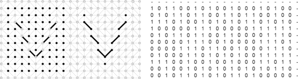
FIGURE 7.15 The states of switches are uniquely defined or can be chosen arbitrarily in most cases. Only in a few flip-flop cases (12 in this example) are the switches set using the templates shown in Figure 7.16. The binary matrix S on the right represents the states of all of the switches.

FIGURE 7.16 s-Adjacencies for the switch state matrix shown on the right in Figure 7.15.
In terms of s-adjacency, we can define s-curves, s-separation (using s-paths), and region (s)-adjacency graphs. Because an s-adjacency graph is planar, Theorems 7.6 and 7.7 are valid when we use s-adjacency:
The proofs of these theorems are the same as the proofs of the corresponding theorems for the good pair (6,6), which defines a special case of s-adjacency. Figure 7.17 shows (on the left) a simple s-curve and (on the right) a partition into regions defined by a subset M.

7.4 Surfaces in the Euclidean Topology
A topologic space S is called locally compact iff every p ∈ S has a topologic neighborhood with a closure that is compact.
Evidently, En is an n-manifold and so is an open n-sphere in En; thus an n-manifold can be bounded or unbounded. A bounded 1-manifold is either a simple (Urysohn-Menger) curve or a simple arc without its endpoints and is homeomorphic to an open line segment. In general, a bounded manifold has an “open frontier.” (We recall that the empty set is also an open set.) If M ⊆ E3 and Uε (p) ∪ M is homeomorphic to three open semicircular areas (see Figure 7.18), p is called a bifurcation point of M. A 2- or 3-manifold cannot have a bifurcation point.

An n-manifold is called hole-free iff it is compact (i.e., bounded and closed).5 For example, the surface of a sphere is a hole-free 2-manifold, and so is the surface of a torus.
This allows us to study triangulations of hole-free 2-manifolds. Let Φ be a homeomorphism of such a 2-manifold M onto a polyhedral surface. Let Z be a triangulation of Φ(M) so that Φ(M) is the union of all of the triangles T ∈ Z. The sets Φ−1(T) define a triangulation of the 2-manifold M that consists of curvilinear triangles, their sides (which are simple arcs), and their vertices (points). This allows us to discuss geometric (particularly simplicial) complexes on curved surfaces.
7.4.2 Surfaces
A Jordan surface (C. Jordan, 1887) is defined by a parameterization that establishes a homeomorphism with the surface of a unit sphere. In picture analysis, we are usually not interested in parameterizations of surfaces. (See Chapter 8 about the geometry of Jordan surfaces.) Instead, we use a topologic definition of a surface that can be compared with the topologic definition of a Urysohn-Menger curve (see Section 7.1.2):
Evidently, S = S• = S° ∪ ϑS, where S• denotes the closure of S. If ϑS = ø, S is called a hole-free surface. A surface is either a hole-free surface or a surface with frontiers. A simple hole-free surface is a hole-free surface that is homeomorphic to the surface of a sphere (i.e., it is a Jordan surface).
The frontier ϑS of a surface S with frontiers is an elementary curve that is a union of pairwise disjoint simple curves. Figure 7.19 shows two examples: the surface of a sphere with a few circular areas removed and the surface of a torus with one circular area removed (a handle). A simple surface with r contours is a surface with frontiers and is homeomorphic to the surface of a sphere with r holes that has frontiers that are pairwise disjoint.

FIGURE 7.19 The surface of a sphere without a few circular areas (left). The surface of a torus without one circular area (right); this surface is called a handle.
In what follows, we assume that any surface with frontiers can be defined by a triangulation (i.e., it is a union of finitely many points, simple arcs, and curvilinear triangles). More generally, we say that a finite or infinite connected graph drawn on a surface S with frontiers defines a tiling of S iff every edge of the graph is on a circuit (encircling a face), there is a vertex at any point at which edges intersect, and ϑS is contained in the union of all of the edges and vertices. (A planar graph was defined based on a drawing on a planar surface. Similarly, a toroidal graph could be defined based on a drawing on a toroidal surface, and so on.) We identify a tiling with its set of faces (2-cells), edges (1-cells), and vertices (0-cells). The side-of relation defines a partial ordering on the set of 0-, 1-, and 2-cells of a tiling. Thus, it follows:
Triangulations are examples of tilings. A tiling is called regular iff every face of the tiling is an n-gon (a simple polygon that has n ≥ 1 vertices on its frontier) and every vertex is incident with exactly k ≥ 1 faces.
Example 7.1
In accordance with %Theorem 7.10, a Jordan surface is homeomorphic to a polyhedron. Suppose the faces and vertices of this polyhedron define a finite regular tiling. By the Descartes-Euler polyhedron theorem, we have α0 –α1 +α2 = 2. For a regular tiling, we have 2α1 = kα0 (because each vertex is incident with k edges and an edge is defined by two vertices) and 2α1 = nα2 (because each edge is incident with two faces and each face has n edges). Hence we have the following:
The only solutions to this Diophantine equation are given by the five regular polyhedra. In particular, there are no solutions for α1 > 30; thus no regular finite tiling on a Jordan surface can be of interest for defining a picture grid. There are triangulations (n = 3) of a Jordan surface that have α1 > 30, but the degrees of the vertices of these triangulations cannot have a constant value. Interestingly, there are finite regular tilings on the surface of a torus (which is a hole-free 2-manifold) in which the size of α1 is not limited. Thus nontrivial picture grids can be defined on the surface of a torus but not on the surface of a sphere.
Let Z be a triangulation of a hole-free surface or of a surface with frontiers. The relation ≤ defined by the side-of relationship defines a poset that has an Aleksandrov topology. Let UZ (t) denote the smallest neighborhood of t in Z. For example, the smallest neighborhood UZ (p) of a vertex p in Z contains p and may also contain curvilinear triangles pr1r2 and simple arcs pq. The set of vertices q of these arcs and the set of arcs r1r2 of these triangles define a subcomplex ϑZ (p) called the frontier of UZ (p). UZ(p) is called cyclic iff the union of the simple arcs on its frontier ϑZ (p) is a simple curve; otherwise it is called acyclic. Figure 7.20 shows examples. If UZ(p) is cyclic, it is homeomorphic to a closed disk.
P. S. Aleksandrov (1956) proved several theorems about surface triangulations. We cite three of them:
(i) Z is a triangulation of a hole-free surface iff Z is connected and UZ (p) is cyclic for all vertices p of Z.
(ii) Every simple arc in a triangulation Z of a hole-free surface is a side of exactly two triangles in Z.
(For more about the term “strongly connected,” see the end of Section 6.4.3.) Note that (i) gives a local criterion for testing a global property of a triangulation. It can be used, for example, in a marching cubes algorithm to test whether the isosurface generated by the algorithm is without frontiers (hole-free). According to (ii), “modulo 2” homology theory (see the definition of a chain frontier in Section 6.4.5) can be applied to triangulations of surfaces.
7.4.3 Orientable surfaces
A simple arc with endpoints p and q will be denoted by [p, q] and the corresponding open arc by (p, q). [p, q] is homeomorphic to the closed interval [0,1]. The direction of [p, q] is defined by a homeomorphism Φ:[0,1] → [p, q] such that Φ(0)=p and Φ(1) = q. Let the following be true where r1, r2 ∈ [p, q]:
The relation ![]() defines an order on [p, q]; it can be shown that this order is independent of the homeomorphism Φ. Analogously, we can define a direction on a simple curve such as the frontier of a triangle. A direction on a simple curve induces a direction on the simple arcs contained in the curve.
defines an order on [p, q]; it can be shown that this order is independent of the homeomorphism Φ. Analogously, we can define a direction on a simple curve such as the frontier of a triangle. A direction on a simple curve induces a direction on the simple arcs contained in the curve.
An oriented triangle is a triangle with a direction on its frontier (e.g., clockwise, counterclockwise), that is called the orientation of the triangle. The orientation of a triangle induces orientations of its sides. Two triangles in a triangulation that have a common side are coherently oriented if they induce opposite orientations on their common side. These standard definitions in combinatorial topology are consistent with our definitions of oriented adjacency graphs in Section 4.3.
If Z is a strongly connected orientable triangulation, the orientation of any triangle of Z determines the orientation of all of Z; hence any such triangulation has exactly two orientations. (We had an analogous result for orientations on the regular 2D grid [see Figure 4.19]: Only options (A) and (F) could be used.)
The fact that orientability does not depend on the triangulation allows us to define a surface as orientable iff it has an orientable triangulation. Theorem 7.11 implies that orientability of a surface is a topologic invariant.
Example 7.2
(J.B. Listing, 1861; A.F. Möbius, 1865) A famous example of a nonorientable surface is the Listing band originally described by J.B. Listing in 1861; see Figure 7.21. (This band is usually called the “Möbius band ” after A.F. Möbius, who discovered it independently in 1865. An example of an isothetic Listing band is shown in Figure 7.22.) The frontier of the Listing band is a simple curve that is homeomorphic to a circle. We can obtain a hole-free surface that is not a Jordan surface by starting with the surface of a sphere from which some circular areas have been removed (Figure 7.19) and identifying the frontier of each circular area with the frontier of a Listing band.

FIGURE 7.21 A Listing band as drawn by O. Veblen in 1922. The rectangle (left) is transformed into the Listing band (right) if a corresponds to c and b to d.

FIGURE 7.22 An isothetic Listing band [632].
This example illustrates the possible topologic complexity of surfaces.6 We can also cover any of the holes with copies of a handle (a torus with a hole). This process of gluing a frontier of one surface to a frontier of another requires the two frontiers to be homeomorphic, and the result may also depend on the orientations of the frontiers. For example, we can glue the frontiers of two handles together and obtain a hole-free surface that is homeomorphic to the result of gluing two handles to the frontiers of a sphere with two holes.
7.4.4 The connectivity and genus of a surface
Let α0,α1, and α2 be the numbers of points, simple arcs, and curvilinear triangles in a triangulation Z of a surface. The Euler characteristic of Z is x(Z) = α0 –α1 +α2.
This theorem allows us to speak about “the ” Euler characteristic of a surface, which is a topologic invariant. It also follows that the Euler characteristic of any finite tiling of a surface (e.g., a regular tiling), where α0,α1, and α2 are the numbers of vertices, edges and faces of the tiling, is equal to x(S).
For example, each face of a cube can be triangulated into two triangles. This results in 8 vertices, 18 edges, and 12 triangles so that the Euler characteristic of the triangulation is 2. The surface of a sphere can be, for example, subdivided into four curvilinear triangles; this results in 4 vertices and 6 simple arcs so that the Euler characteristic is again 2. This also follows from Theorem 7.12, because the surfaces of the cube and the sphere are homeomorphic.
We say that a one-dimensional closed subcomplex M of a triangulation Z of a surface does not separate Z iff the open subcomplex Z/M is strongly connected. The connectivity q(Z) of Z is the n for which Z has a closed one-dimensional subcomplex of connectivity n that does not separate Z.
We recall that the Poincaré formula (Equation 6.6) for S is as follows:
For a hole-free surface S, we have β0(S) = 1 (because S is connected) and β2(S) = 1 (because there exists a triangulation of S that forms a cycle; see (i) at the end of Section 7.4.2), and S is not contractible into a single point. Hence we have the following, where Z is any triangulation of S:
Z defines a graph G (a one-dimensional Euclidean complex), and we have x(Z) = 1 + x(G) = 2 –β1(G).β1(S) is called the connectivity of S. Finite triangulations or square tilings of homeomorphic surfaces have the same connectivities. We can therefore speak about “the ” connectivity of a surface; it is a topologic invariant.
For example, the Euler characteristic of a sphere with r holes is 2 – r. Indeed, we saw above that the sphere has Euler characteristic 2. Every deletion of a triangle from the triangulation such that its vertices and edges remain in the triangulation decreases the Euler characteristic by 1.
From the topology of complexes (see [639]), we know that the Betti number β1(S) of a hole-free orientable surface is even and is equal to twice the genus of the surface (see Section 1.2.6), and that, for a hole-free nonorientable surface, it is odd and equal to the genus plus 1. For example, if we start with a sphere with r = 0 holes and identify the frontier of each hole with the frontier of a Listing band, we obtain a hole-free nonorientable surface Lr of genus r; if we identify the frontier of each hole with the frontier of a handle, we obtain a hole-free orientable surface Sr of genus r. Any hole-free surface S has the same Euler characteristic (or genus) as one of the surfaces Sr (if S is orientable) or Lr (if it is nonorientable).
7.4.5 Separation theorems
The separation theorems for planar simple curves discussed in Section 7.1.5 were generalized around 1900, first to 3D space and then to n dimensions.
A Jordan curve is the homeomorphic image of a circle, and a Jordan surface is the homeomorphic image of the surface of a sphere. This was generalized by L.E.J. Brouwer in 1912 to the n-dimensional case. He defined a Jordan manifold in Rn (n ≥ 2) as the homeomorphic image of a closed (n − 1)-dimensional sphere and proved the following:
In a paper published that same year, O. Veblen showed (without using a parameterization) that the surface of a simple bounded n-dimensional polyhedron decomposes the n-dimensional space (defined by axioms) into two connected subsets, that it is the frontier of each of the subsets, and that any polygonal arc that joins a point of one subset to a point of the other contains a point of the polyhedron.
7.5 Surfaces and Separations in 3D Grids
Surfaces in picture analysis are defined by sets of voxels. Surfaces in the grid can be characterized as 2D sets of voxels in a 3D adjacency grid or as 2D Euclidean complexes of marginal cells (2-, 1-, and 0-cells given by the frontier of a region). In the first case, we assume the grid point model.
7.5.1 Surfaces in the grid point model
p is called an (α,α’) surface voxel of S ⊆ Z3, where (α,α’) = (26,6) (the (6,26) case can be treated analogously), iff the following are true:
a) A26(p) ∩ S has exactly one α-component that is α-adjacent to p.
b) ![]() has exactly two α′ -components Cp, Dp that are α′-adjacent to p.
has exactly two α′ -components Cp, Dp that are α′-adjacent to p.
An α-connected set S ⊆ Z3 is called an α-surface iff every p ∈ S is an (α,α′) surface voxel. Let N(p) be a 5 × 5 × 5 block of voxels centered at p. In [747], a surface voxel p is called orientable if ![]() has exactly two α’-components that are α’-adjacent to p, and an α-connected set S is called an α-surface if it consists entirely of orientable (α,α′) surface voxels; however, it was shown in [841] and [840] that the assumption of orientability was unnecessary.
has exactly two α’-components that are α’-adjacent to p, and an α-connected set S is called an α-surface if it consists entirely of orientable (α,α′) surface voxels; however, it was shown in [841] and [840] that the assumption of orientability was unnecessary.
For (α, α’) = (26,6), we have the following:
p =(i,j,k) ∈ S is called a border point of S iff it has only one 26-neighbor in {(x,y,z) ∈ S : x = i}, {(x,y,z) ∈ S : y = j}, or {(x,y,z) ∈ S : z = k}; it is called an inner point of S iff it is not a border point. A 26-surface is called simple iff it has no border points. A simple 26-surface can be unbounded, or it can be bounded and hole-free. A bounded digital surface with border points that are 26-connected is called a digital surface patch.
If S is an α-surface, every voxel of S is adjacent to both components of ![]() . For α-curves in Z2 ((α,α’) = (4,8) or (8,4)), the converse is also true: if S is α-connected,
. For α-curves in Z2 ((α,α’) = (4,8) or (8,4)), the converse is also true: if S is α-connected, ![]() has two α’-components, and every pixel of S is adjacent to both of these components, then S is an α-curve (see Exercise 5 in Section 7.6); however, the analogous statement about α-surfaces is not true, because a surface can touch itself without affecting the connectedness of its complement.
has two α’-components, and every pixel of S is adjacent to both of these components, then S is an α-curve (see Exercise 5 in Section 7.6); however, the analogous statement about α-surfaces is not true, because a surface can touch itself without affecting the connectedness of its complement.
In the example in Table 7.1, the 1s are 6-connected, the (nonbackground) 0s are 26-connected, and every 1 is adjacent to both 26-components of 0s (the central 1s in the third and fifth planes are adjacent to background 0s in the fourth plane), but the central 1 in the fourth plane is adjacent to four components of 0s in its 27-neighborhood.

7.5.2 Surfaces in the grid cell topology
We recall that a connected set in [Cn, ≤] is 2D if it contains at least one 2 × 2 block of cells (e.g., one 2-cell with two incident 1-cells and one 0-cell; see Proposition 6.2). In a discrete grid, we cannot ask for a one-dimensional separation of each point of a set from the rest of the set. A hole-free surface (e.g., the frontier of a simply connected 6-region) can be transformed into a region of a 2D incidence pseudograph by removing a few of its cells. Note that we are using “6-simply connected region ” and “simply connected 6-region ” as equivalent. Cells in the frontier of this 2D region cannot be separated from the rest of the region by one-dimensional circuits of cells. An important feature of Definition 6.7 is that it allows a definition of “2D at cell c ” without requiring the existence of such one-dimensional separations.
Any 6-region of voxels in the grid cell model is a finite union of simply connected 6-regions. Due to 18- or 26-adjacencies, there may be “touchings ” between voxels of a 6-region. A 6-connected region corresponds with an open 2-region in the grid cell topology [C3, I, dim]. A simply 6-connected region M is defined by a simply connected geometric representation Mg in the incidence grid; see Definition 7.8. We characterize the surface ϑ(M) of a simply connected 6-region by the frontier ∂Mg of the geometric representation Mg of the corresponding open 2-region.
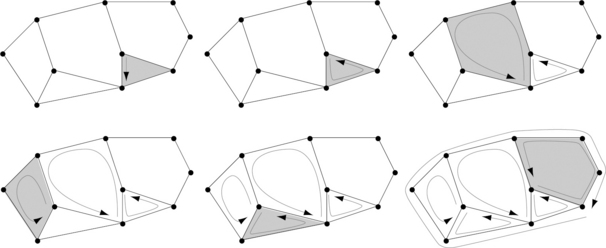
This proposition guarantees the existence of an orientation on ∂Mg that can be “copied ” (from each face of a cube in ∂Mg to the corresponding face of the cube in ϑM) onto the surface ϑ(M). Moreover, an orientation on such a surface ∂Mg is easy to construct. Assume that the simple surface is mapped into a finite 3-strong planar graph G (see Steinitz’s Theorem in Section 4.2.2). An orientation of all faces of G (including the unbounded face) can be defined by choosing an orientation for any edge in any face; this defines a cyclic orientation in the face. Any edge in any face that is edge-adjacent to an already oriented face is then oriented in the opposite direction, thereby defining an orientation in this new face (see Figure 7.23). There are only two possible orientations for the first edge; hence there are only two possible orientations for G. (For the construction of the orientation, it is actually sufficient that G be a planar 2-strong graph.)
Now consider the preimage of G on the surface ∂Mg, which defines a tiling of ∂Mg. We map the constructed orientation of G onto this tiling and obtain an orientable Euclidean complex; its faces are polygons, and their proper sides are their edges and vertices. There are only two possible orientations for this surface complex.
Now consider a purely n-dimensional simplicial complex that is (n − 1)-connected (i.e., between any two n-simplexes c1 and c2 and there is a path of n-simplexes from c1 to c2 such that any two consecutive n-simplexes on the path share an (n − 1)-simplex). We can define one of the two possible orientations for this simplicial complex by propagating orientations as in the planar case: choose an initial n-simplex c0 and an initial edge p0p1 in one of the 2-simplexes (triangles) that bound c0, and choose one of the two possible orientations of this edge. This defines oriented triangles p0p1p2, p1p3p2, p2p3p0, and p3p1p0, which are the four 2-sides of a (now oriented) tetrahedron p0p1p2p3. For n> 3, we would continue by orienting another 3-side of c0 that is 2-adjacent to p0p1p2p3 and that inherits its orientation by inverting the orientation on the joint 2-side. For n = 3, we have c0 = p0p1p2p3, and we propagate orientations to all of the 2-adjacent tetrahedra. For example, if p0p1p2 is shared with the 2-adjacent tetrahedron c1, we have the orientation p2p1p0 for this face on c1,so c1 = p2p1p0p4 where p4 is the fourth vertex of c1.
If we have a purely n-dimensional (n − 1)-connected grid cell complex, we can propagate orientations in the same way. We start with an edge e0 = p0p1; this defines an orientation for a face f0 = e0e1e2e3. Let f1 be an edge-adjacent face, for example, f0 ∩ f1 = e0. Then ![]() where
where ![]() . We continue orienting all of the 2-faces of a grid cube c0, for example, in the order f0f1f2f3f4f5, which defines a Hamilton cycle through the faces (see Figure 5.27). (Note that we cannot represent grid cells solely by sequences of vertices as we did in case of simplicial cells, because the order of the vertices is now relevant.) We continue with a cube c1 that is face-adjacent to c0, for example
. We continue orienting all of the 2-faces of a grid cube c0, for example, in the order f0f1f2f3f4f5, which defines a Hamilton cycle through the faces (see Figure 5.27). (Note that we cannot represent grid cells solely by sequences of vertices as we did in case of simplicial cells, because the order of the vertices is now relevant.) We continue with a cube c1 that is face-adjacent to c0, for example ![]() with
with ![]() . The process continues until all of the edges, faces, cubes, and so forth of the complex have been oriented. In fact, we can define an orientation on all of Cn in this way, and any oriented n-dimensional grid cell complex is then just a subcomplex of Cn equipped with the chosen default orientation.
. The process continues until all of the edges, faces, cubes, and so forth of the complex have been oriented. In fact, we can define an orientation on all of Cn in this way, and any oriented n-dimensional grid cell complex is then just a subcomplex of Cn equipped with the chosen default orientation.
For both simplicial and grid cell complexes, there are only two possible orientations for any (n − 1)-connected purely n-dimensional complex. In the case of the simplicial complex K, we choose an orientation for the triangulated surface ϑ(K). In the case of the grid cell complex G, it defines an orientation for the square tiling of the surface ϑ(G).
From Proposition 7.6, we know that the frontier ∂Gg of the geometric representation of an open 2-region ![]() (a union of finitely many simply connected 6-regions) is always hole-free and orientable. This frontier is bounded, because a region is finite, and it is closed because, for every 2-cell c in the frontier ϑG, all of the 1-cells and 0-cells incident with c are in the frontier, and, for every 1-cell c’ in the frontier, all of the 0-cells incident with c’ are in the frontier.
(a union of finitely many simply connected 6-regions) is always hole-free and orientable. This frontier is bounded, because a region is finite, and it is closed because, for every 2-cell c in the frontier ϑG, all of the 1-cells and 0-cells incident with c are in the frontier, and, for every 1-cell c’ in the frontier, all of the 0-cells incident with c’ are in the frontier.
The frontier ϑ(G) of a region ![]() can be represented in the frontier grid; see Definition 7.4 for n = 3. This defines an isothetic polyhedron (see Chapter 8). The separation theorems of Euclidean topology apply to these polyhedra.
can be represented in the frontier grid; see Definition 7.4 for n = 3. This defines an isothetic polyhedron (see Chapter 8). The separation theorems of Euclidean topology apply to these polyhedra.
7.5.3 Separations in adjacency grids
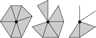
M ⊆ Z3 is called an (α,β)-separator iff M is α-connected, M divides Z3/M into (exactly) two β-components, and there exists a p ∈ M such that Z3/(M/{p}) = (Z3/M) R {p} is β-connected.
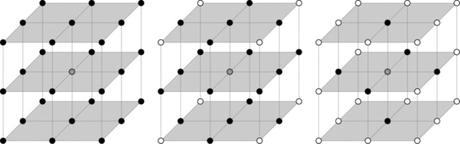
In Figure 7.24, the set M1 on the left is a (2,2)-, (2,1)-, and (2,0)-separator. If any voxel is removed from M1, its complementary set becomes 0-connected. There also exist voxels in M1 such that removal of one of them makes the complementary set 1- or 2-connected. The set M2 in the middle is a (1,2)- and (1,1)-separator, and the set M2 on the right is a (0,2)-separator.
(α,β)- and (β,α)-separators exist for (α,β) = (0,2), (2,0), (1,2), (2,1), and (1,1). However, there are some difficulties with (α,β) = (1,1). For a 3D connected set M, we expect that x(M) = 1 – t + c, where t is the number of tunnels and c the number of cavities. For the set M in Figure 7.25, there is no cavity and one tunnel, so we expect that x(M) = 1 − 1 + 0 = 0. However, the set M0 of voxels of M that have x-coordinate 0 is simply 1-connected, so x(M0) = 1. Let M + (M−) be the set of voxels of M that have nonnegative (nonpositive) x-coordinates. By symmetry, we have x(M +) = x(M−) = a. However, because M0 = M + ∩ M− and M = M + R M−, we must have x (M) = x (M +) + x(M−) – x(M0) = 2a – 1 ≠ 0. (Here we have used a sum formula for the Euler characteristics of unions of Euclidean complexes; it is true for arbitrary unions of finite complexes.) Note that we would encounter the same difficulty for (α,β) = (0,0.), but this case is not on our list of separators. (0,2), (2,0), (1,2), and (2,1) are considered to be “good pairs of separators ” in the grid cell model; they correspond with (6,26), (26,6), (6,18), and (18,6) in the grid point model.

The empty set is α-connected; it follows that M is not α-separating in itself. If S = M R {p}, then M can also not be α-separating in S. Let p and q be any two points in Zn/M that are not α-connected; then M is α-separating in M R {p, q}.
In the grid cell model, we have α, β ∈ {0,1,2}, and M has β-gaps iff it is α-separating in some superset of S but not β-separating in S for α>β.
Figure 7.26 illustrates gaps. An (α,β)-se ρarator M does not have β-gaps. See Exercise 12 for more about gaps in digital lines and Section 11.2.4 for more about gaps in digital planes.

FIGURE 7.26 From left to right: for n = 2, a 0-gap and a 1-gap; for n = 3, two 0-gaps, a 1-gap, and two 2-gaps [130].
7.6 Exercises
1. Prove that the property of being a (Urysohn-Menger) curve is a topologic invariant in the Euclidean plane.
2. Let γ be a simple (Urysohn-Menger) curve on the surface S of a sphere. Prove that the complementary set S/γ consists of two open subsets of S with the common frontier γ.
3. Classify all of the elementary curves (“letters ”) in Figure 7.4 with respect to topologic equivalence.
4. Suppose n> 0 finite connected polygonal chains in E2 start at p, end at q ≠ p, and intersect only at p and q. Prove that the chains partition E2 into n disjoint sets.
5. Prove that a set of grid points C is a simple 4- (8-)curve iff C is 4- (8-)connected and every pixel of C is 4- (8-)adjacent to exactly two other pixels of C.
6. Prove that a subset of Z2 cannot be both a 4-curve and an 8-curve and that a subset of Z3 cannot be both a 6-surface and a 26-surface.
7. If the paths shown in Figure 7.11 are regarded as simple curves in the poset topology of [C2, ≤], is it possible that they do not intersect?
8. Prove that, if a 4-component C of 1s and an 8-component D of 0s (or vice versa) in a binary picture are 8-adjacent, they are also 4-adjacent, and either D 4-surrounds C (i.e., D 4-separates C from the infinite background component B)or C 8-surrounds D (i.e., C 8-separates D from B).
9. Suppose the chessboard pattern in Exercise 4 (ii) in Section 1.3 is digitized into an 8 × 8 binary picture. What are its components if we use good pairs (4,8), (8,4), and (6,6)? How do these results compare with your discussion of Exercise 4 (ii) in Section 1.3? Can you specify a switch state matrix S such that all of the “black pixels ” in the upper four rows and all of the “white pixels ” in the lower four rows are s-connected?

10. Prove that (6,6) is a good pair for Z2.
11. Define a set of 4 × 4 templates for choosing the values of flip-flop switches so as to give preference to line-like patterns, whether the lines are black or white.
12. Let S be a set of voxels in the grid cell model. A 2-cell that is a common face of a voxel of S and a voxel of ![]() is called a surface pixel of S. Two surface pixels are called edge-adjacent if they share a 1-cell, and they are called vertex-adjacent if they share a 0-cell but not a 1-cell. Prove that any surface pixel of S must be edge-adjacent to an even number of surface pixels of S, that this number must be between 4 and 12, and that a surface pixel of S can be vertex-adjacent to at most 20 surface pixels of S.
is called a surface pixel of S. Two surface pixels are called edge-adjacent if they share a 1-cell, and they are called vertex-adjacent if they share a 0-cell but not a 1-cell. Prove that any surface pixel of S must be edge-adjacent to an even number of surface pixels of S, that this number must be between 4 and 12, and that a surface pixel of S can be vertex-adjacent to at most 20 surface pixels of S.
13. Two surface pixels (see Exercise 12 above) are called strongly edge-adjacent if they are edge-adjacent and are surface pixels of voxels of S with intrinsic 6-distances apart that are at most 3. Prove that a surface pixel of S is strongly edge-adjacent to exactly four surface pixels of S. Prove that, if T is a maximal strongly edge-connected set of surface pixels of S, then there exist a 6-component U of S and an 18-component V of ![]() such that T is the set of surface pixels that are common faces of voxels in U with voxels in V.
such that T is the set of surface pixels that are common faces of voxels in U with voxels in V.
14. What are the Euler characteristic and genus of the surface of a sphere, a torus, a handle, and a Listing band?
15. Let S1 and S2 be two surfaces with frontiers. Glue S1 and S2 together by identifying a simple curve in ϑS1 with a simple curve in ϑS2. Prove that the resulting surface has Euler characteristic χ(S1) + χ(S2).
16. Show that a handle has a tiling defined by one vertex, three edges, and one face.
17. Prove that any regular tiling of the Euclidean plane is topologically equivalent to a regular tiling of the plane in which the set of vertices coincides with Z2.
18. Prove that the Euclidean plane allows regular tilings (with α1 = N0) only for n = k = 4, n = 3, and k = 6, or n = 6 and k = 3.
19. Prove that the graph of a regular tiling of the surface of a sphere is homeomorphic to one of the five Platonic graphs (tetrahedron, octahedron, icosahedron, hexahedron, or dodecahedron) or to a graph defined either by n = 2 and α1 = k ≥ 2 or by n = α1 > 2 and k = 2.
20. Prove that the surface of a torus has regular tilings (with α1 < N0) for only n = k = 4, n = 3, and k = 6, and n = 6, and k = 3.
21. Suppose there exists a regular tiling on a hole-free surface with n = 5 and k = 4. Prove that, if the number of faces of the tiling is not a multiple of 8, the surface is not orientable.
22. Prove that a surface with frontiers is not simply connected if its frontiers consist of more than one simple curve.
7.7 Commented Bibliography
For the original work on Urysohn-Menger curves, see [725, 1081, 1082]. Curves are studied in [798]; for a review of their history, see also [1006]. Curves and complexes are discussed in [9,10]; see also %Theorem 7.1. %Theorem 7.3 was proved in [1085] (see also [483]), %Theorem 7.4 in [962] and [138], and %Theorem 7.5 in [1030]. For Brouwer’s work on separation theorems, see [138,139]. For Definition 7.12 and Theorems 7.11 and 7.12, see [9]. For %Theorem 7.10, see [358].
For the topology of surfaces, see [9, 10, 639]. %Theorem 7.13 was published in [139], and the cited work of O. Veblen was published in [1086]. Listing’s band was published in [660]; its independent publication by Möbius in [734] came four years later. Figure 7.21 is from [1087]. For a digital formulation of %Theorem 7.13 for the 3D grid cell topology, see [587].
Characterizations of simple arcs and curves in 2D adjacency grids are given in [882]; see also [1029]. The term “good pair” was introduced in [569]. See [576] for a discussion of other pairs of adjacencies, and see [336] for an axiomatic treatment of good pairs. %Theorem 7.7 is proved in [884]. Definitions of digital surfaces based on the (6,26)-adjacency grid are studied in [211, 689, 747, 841], related region adjacency graphs in [894], and calculations of 3D Euler characteristics (with subsequent studies of homotopy) in [694]. For “digital Urysohn curves ” in 2D adjacency grids, see [1112]. Curves and surfaces in the 1- and 2-adjacency grid are discussed in [1005]. Adjacencies between convex cells (generalizing the regular orthogonal grid cell model) are studied in [942, 943, 944]. For other work on digitized curves and boundaries, see [915, 1121].
[632] shows that “simply connected ” and “contractible ” are locally computable properties in 2D good pair grids but not in 3D good pair grids. (The Euler characteristic is locally computable; see Exercise 6 in Section 6.5 and [577] for a related review.) Local property detection in “grid topologies ” that are not necessarily defined on regular grids was studied in [320]. Local property calculation based on incidence matrices of graphs was studied in [474]. [81] characterizes surfaces in 3D adjacency grids by “simple ” global properties, and [690] studies equivalent local characterizations. See [1059] for connectivities of 3 × 3 × 3 voxel sets and [578] for Euler characteristics in (4,4)- or (8,8)-adjacency grids.
The approximation of n-dimensional manifolds by graphs is studied in [1060, 1061], with a special focus on topologic properties of such graphs defined by homotopy and on homology or cohomology groups. Definition 7.5 is from [511]. The approximation of boundaries of finite sets of grid points (in n dimensions) based on “continuous analogs ” was proposed and studied in [613]. [496] discusses local topologic configurations (stars) for surfaces in incidence grids. Digital surfaces in the context of arithmetic geometry [848] were studied in [131].
The results of [747] are generalized in [573] to all α and α’ in {6, 18, 26} except α = α’ = 6. A Jordan surface theorem for the Khalimsky topology is proved in [587]. [685] introduces a general classification of the voxels of a set S using the numbers of components of S and ![]() in the neighborhood of the voxel. For discrete combinatorial surfaces, see [339]. For obtaining α-surfaces by the digitization of surfaces in E3, see [209] and [211]. It is proved in [688] that there is no local characterization of 26-connected subsets S of Z3 such that
in the neighborhood of the voxel. For discrete combinatorial surfaces, see [339]. For obtaining α-surfaces by the digitization of surfaces in E3, see [209] and [211]. It is proved in [688] that there is no local characterization of 26-connected subsets S of Z3 such that ![]() consists of two 6-components and every voxel of S is adjacent to both of these components. [689] defines a class of 18-connected surfaces in Z3, proves a Jordan surface theorem for these surfaces, and studies their relationship to the surfaces defined in [747]. [80] introduces a class of strong surfaces and proves that both the 26-connected surfaces of [747] and the 18-connected surfaces of [689] are strong. [688] and [690] give local characterizations of strong surfaces. For 6-surfaces, see [194].
consists of two 6-components and every voxel of S is adjacent to both of these components. [689] defines a class of 18-connected surfaces in Z3, proves a Jordan surface theorem for these surfaces, and studies their relationship to the surfaces defined in [747]. [80] introduces a class of strong surfaces and proves that both the 26-connected surfaces of [747] and the 18-connected surfaces of [689] are strong. [688] and [690] give local characterizations of strong surfaces. For 6-surfaces, see [194].
Frontiers in cell complexes (and related topologic concepts such as components and fundamental group) were studied in [11]. For characterizations of and algorithms for curves and surfaces in frontier grids, see [425, 426, 427, 428, 594, 596, 917, 1075, 1076, 1078]. G.T. Herman and J.K. Udupa used frontiers in the grid cell model, and V. Kovalevsky generalized these studies using the model of topologic abstract complexes that was briefly introduced in Section 6.4.4. Our definitions of curves in incidence grids resemble work in [217].
Gaps were introduced and studied in [23, 848] using the term “tunnel ” instead of “gap.” This was later generalized in [130, 133] to a definition of “j-tunnels ” in arbitrary sets of grid points. This notion of a tunnel is not the same as the tunnels defined in Section 6.4.5. [130, 133] also introduced and studied k-separability.
For a review of curves and surfaces in digital topology, see [577], and, more recently, [569]. Exercise 12 and Example 7.1 are from [100]
1For the first appearance of the term “Jordan curve,” see [787]: “By a Jordan curve is meant a curve of the general class of continuous curves without multiple points, considered by Jordan, Cours d’Analyse, vol. I, 2d edition, 1893, p. 90…”
2For a first use of the term “Jordan curve theorem,” see [1129]; D.W. Woodard was the second African American who received a PhD in mathematics.
3This notation is consistent with that for Gauss digitization.
5We use the term “hole-free manifold ” instead of “closed manifold ” to avoid confusion when we discuss closed complexes defined by tilings of manifolds.
6Surfaces will be further discussed in Chapters 8 (surface geometry), 11 (planarity), and 12 (estimation of surface area and curvature).