9.1 Summary
The book has three parts: concepts and the background of visual attention (Chapters 1 and 2), computational models and performance benchmarking (Chapters 3, 4, 5 and 6) and applications of visual attention modelling (Chapters 7 and 8).
Chapter 1 in Part I introduces the definition and classification of visual attention, as well as its contributions to visual information processing. Three principal concepts result from intuitional experiments and records of eye movements: (1) Visual attention is in existence universally. (2) Visual attention can be classified into different types: pre-attention, attention and post attention, based on the order of processing stage; bottom-up and top-down attention according to different driving sources – external data driven for bottom-up and internal task (motivation) driven for top-down; parallel and serial attention in the light of different processing manners; overt and covert attention based on whether there is eye movement or not. (3) Change blindness and inhibition of return exist in visual attention.
The foundation on which to build computational attention models is presented in Chapter 2 of Part I. The basis of biology comes from two aspects: one is from physiology and anatomy, and the other from psychological and neuroscience studies. In addition, the ground of engineering is from the theory of statistical signal processing.
9.1.1 Research Results from Physiology and Anatomy
Visual information processing in low-level cortex (from retina to primary cortex V1 area) has the following five major characteristics:
The visual information processing from primary cortex (V1) to other areas (e.g., V2–V5 areas) in the high level of the brain is complex and less known in general. Some well-known findings related to visual attention are as follows.
There are three other processing rules in the brain: (a) competition among cells occurs in all areas in the visual cortex; (b) normalization – the response of cells is that each cell's response is divided by the activity from a large number of cortical cells that extracts the same feature, so the cell's activity within larger activity energy is inhibited; (c) whitening in the different frequency band (or centre–surround processing) of ganglion cells replenishes the decline of the spatial frequency spectrum in natural scenes, resulting in a whitened response spectrum.
9.1.2 Research from Psychology and Neuroscience
There are many research achievements in psychology and neuroscience for visual attention. This book mainly introduces the two most famous theories – feature integration theory and guided search theory – because these two theories are the basis of the saliency map models that most applications in the engineering area adopt. With the temporal tagging hypothesis at the neuronal level, synchronized oscillation theory has also been presented in Part I, which explains other kinds of feature binding possibilities with time at the neuronal level. We summarize these three theories below.
9.1.3 Theory of Statistical Signal Processing
Experts, engineers and students engaged in computer or signal processing, are no strangers to statistical signal processing. In Part I we have listed three aspects of statistical signal processing, related to the computational models discussed in the book.
9.1.4 Computational Visual Attention Modelling
The signal detection theory, statistical signal estimation and information theory mentioned above have been used in computational saliency models in Part II. Some computational models make use of one or several biological results or rules, while others utilize both biological and statistical signal processing theories.
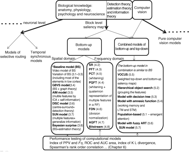
In Part II, bottom-up visual attention models and combined models of bottom-up and top-down were discussed in Chapters 3, 4 and 5. Bottom-up models are discussed separately in the spatial domain and in the frequency domain. Frequency domain models are more suitable for efficient and real-time applications. Each computational model can be analysed with different benchmarking criteria. Of course, different models may be propitious for different purposes or applications. Nevertheless, for a newly created computational model, comparisons are necessary in order to confirm whether a new model has its superiority in different areas of interest. Chapter 6 gives the commonly adopted quantitative criteria that help to test the new or improved visual computational models. Figure 9.1 shows the computational models already presented in Part II and based upon the background knowledge of both biological and information theories in Part I.
Figure 9.1 Summary of computational models in Part II

In Figure 9.1, the top block represents the background knowledge of biology, statistical signal processing and computer vision. Three bold arrows from the top block represent three branches: models described at the neuronal level, pure computer vision based models and saliency map models which is the main topic of this book. The dotted lines at both sides denote that more branches and models (e.g., pure computer vision ones) are possible. Since this book mainly discusses saliency models based on block description, the mid bold arrowhead grows to the areas illuminated in Part II. The computational model we refer to as the saliency map model indicates that the computation result is a saliency map with topography. A saliency map can guide the visual attention in the input visual field and the highest peak in the saliency map is the attention focus. These models listed under the middle arrow have been presented in Part II, and the corresponding section of each computational model is listed in Figure 9.1 for convenience of the reader.
9.1.4.1 Bottom-up Computational Models
A typical model with wide use among all the computational models is the baseline (BS) bottom-up model in the spatial domain (see the left block below bottom-up models in Figure 9.1), as presented in Section 3.1. The reasons are: (1) the BS model simulates the four main related functionalities of physiology and anatomy: multiscale feature extraction using image pyramid, centre–surround operation between scales combination across scales and feature channels, and two processing rules (i.e., competition (WTA in saliency map), and normalization for each feature map, compliant with the basic hypotheses in FIT and GS); (2) Most computational saliency map models (both bottom-up, and top-down combined with bottom-up models in the spatial domain) adopt the core of the BS model as a part of the models; (3) it is regarded as a classical model in the literature and the newly created models often compare the performance with that of the BS model.
Other models of bottom-up in the spatial domain, such as GBVS, AIM, DISC, SUN and Bayesian surprise, combine graph theory, information theory and signal processing theory with biological concepts and rules in order to obtain better results.
Frequency domain models are listed in the middle block below bottom-up models in Figure 9.1. Although the models in the frequency domain seem to be little related to the biological basis, uniform amplitude spectrum in PFT, PQFT and PCT just tallies with whitening in different frequency bands of the ganglion cells in the retina. In the FDN model, the three computational stages in the BS model of the spatial domain can be thought of as corresponding to processing in the frequency domain: various features extraction in BS is equivalent to frequency band segmentation in the frequency domain; normalization for each feature map in BS corresponds to division normalization in each segmented frequency band; the combination across scales and feature channels in BS relates to the inverse transform from the frequency domain to the spatial domain. AQFT and bitstream models based on image patches concern the centre–surround difference between patches, and the AQFT makes use of eccentricity of visual acuity on the retina. Moreover, the computational results (saliency maps) of frequency domain models can not only fit natural images, but also fit most image paradigms in psychological experiments that cannot be handled by many pure computer vision based attention models (see Section 9.2 below). In addition, the models in the frequency domain have fast processing speed and can meet the requirements of real-time applications.
9.1.4.2 Combining of Bottom-up and Top-down Computational Models
The right block under combined models in Figure 9.1 lists all the computational models with top-down bias in this book. In combining bottom-up and top-down computational models, the bottom-up part of almost all models uses or partly uses the core of the BS model, and the top-down part often adopts computer vision or neural network based models. The simplest model among them is the VOCUS model in which top-down information is weighted on the feature map with a high degree of separation between the object region and no-object regions, and the integration between top-down and bottom-up processing is accomplished by another weighting process. This is similar to the GS model (GS 2.0). In a hierarchical object search model, grouping of features used in a pure computer vision approach is considered, and the top-down instruction is added by human intervention to complete the search. The three models listed in top-down bias block of Figure 9.1 are the model with decision tree, the model with amnesic function and the population based model (the cell population pattern represents the feature in Section 5.1) that use working memory (i.e., short- and long-term memory) to store top-down knowledge. The memories in models with decision tree and amnesic function are respectively represented by decision tree and amnesic IHDR tree that are often used in object recognition in computer vision. In population based models, the working memory contains the target features represented by the population of cells.
The population based model suggests that the attention is the combined result of local dynamics and top-down biases in large assemblies of neurons involved in competitive interactions. This computational model is most complete among all recommended models in Part II since it includes feature extraction, feature update in feature space (levels 1 and 2), neurons population coding as low-level cortex, learning in working memory and object matching in high-level cortex, inhibition of return (IoR) and the eye movement. The dynamic process is related to the cell activity in the feature space and prior knowledge influence. This model belongs to one of the emergent attention models classified by the book by Tsotsos [5].
The model with fuzzy ART listed in the top-down bias block of Figure 9.1 uses adaptive resonance theory (ART) in neural networks proposed by [7] as top-down knowledge to separate the attention region and the no-attention regions, and the ART model is classified as one of the early temporal tagging models in the book [5]. The final top-down model is the SUN model, which is the same as the SUN of pure bottom-up in a Bayesian framework, but concerns top-down prior knowledge.
The testing methods including PPV, Fη, ROC, AUC, KL divergence and Spearman's rank order correlation of all computational models mentioned in Part II are introduced in Chapter 6 and are also illustrated in the bottom block of Figure 9.1.
9.1.5 Applications of Visual Attention Models
Part III introduces the applications of visual attention models. Two aspects of applications are demonstrated: applications for computer vision and image processing are presented in Chapters 7 and 8 respectively. The applications in computer vision include object detection and recognition for natural images and satellite imagery, walking robots' localization, landmark recognition and moving object recognition in a robot's walking pathway, and image retrieval. The applications of image processing include the JND model combining visual attention towards a complete visibility threshold, and visual attention model applications in image quality assessment, image and video coding, image resizing and compressive sampling. Figure 9.2 lists the possible applications using visual attention models. Another point to note is that some computational attention models with pure computer vision have been introduced for the applications. They do not have any biological basis but solve an idiographic application such as object detection and image retrieval. In the next section, we can see that although these models possibly cannot detect very simple visual paradigms in psychological experiments, they are useful for some practical situations.
Figure 9.2 Applications of visual attention in Part III

