

i
i
i
i
i
i
i
i
16
Brian Wyvill
Implicit Modeling
Implicit modeling (also known as implicit surfaces) in computer graphics covers
many different methods for defining models. These include skeletal implicit mod-
eling, offset surfaces, level sets, variational surfaces,andalgebraic surfaces.In
this chapter we briefly touch on these methods and describe how to build skeletal
implicit models in more detail. Curves can be defined by implicit equations of the
form
f(x, y)=0.
If we consider a closed curve, such as a circle, with radius r, then the implicit
equation can be written as
f(x, y)=x
2
+ y
2
− r
2
=0. (16.1)
The value of f (x, y) can be positive (outside the circle), negative (inside the
circle), or zero for points precisely on the circle. The equivalent in three dimen-
sions is a closed surface around a set of points that occupy a given volume or
region of space. The volume forms a scalar field, i.e., we can compute a value for
every point and as can be seen for the circle, the negative values are bounded by
the implicit curve or surface. The surface can be visualized as a contour in the
field, connecting points with a particular value such as zero (see Equation (16.1)).
To compute such a surface implies searching through space to find the points that
satisfy the implicit equation; this method is unlikely to lead to an efficient al-
gorithm for circle drawing (and even less likely in three dimensions). This was
perhaps the reason that algorithmic methods for modeling with parametric curves
385

i
i
i
i
i
i
i
i
386 16. Implicit Modeling
and surfaces were investigated before implicit methods; however, there are some
good reasons to develop algorithms to visualize implicit surfaces. Chapter 28
mentions scalar fields in the context of volume visualization. In this chapter we
explore the implications of deriving the data from a modeling process rather than
from a scanner.
Despite the computational overhead of finding the implicit surface, designing
with implicit modeling techniques offers some advantages over other modeling
methods. Many geometric operations are simplified using implicit methods in-
cluding:
• the definition of blends;
• the standard set operations (union, intersection, difference, etc.) of con-
structive solid geometry (CSG);
• functional composition with other implicit functions (e.g., R-functions,
Barthe blends, Ricci blends, and warping);
• inside/outside tests, (e.g., for collision detection).
Visualizing the surfaces can be done either by direct ray tracing using an algorithm
as described in (Kalra & Barr, 1989; Mitchell, 1990; Hart & Baker, 1996; deGroot
& Wyvill, 2005) or by first converting to polygons (Wyvill et al., 1986).
One of the first methods was proposed by Ricci as far back as 1973 (Ricci,
1973), who also introduced CSG in the same paper. Jim Blinn’s algorithm for
Figure 16.1. Blinn’s
Blobby Man 1980.
Image
courtesy Jim Blinn.
finding contours in electron density fields, known as Blobby molecules (J. Blinn,
1982), Nishimura’s Metaballs (Nishimura et al., 1985) and Wyvills’ Soft Ob-
jects (Wyvill et al., 1986) were all early examples of implicit modeling meth-
ods. Jim Blinn’s Blobby Man (see Figure 16.1) was the first rendering of a non-
algebraic implicit model.
16.1 Implicit Functions, Skeletal Primitives
and Summation Blending
In the context of modeling an implicit function is defined as a function f applied
to a point p ∈ E
3
yielding a scalar value ∈ R.
The implicit function f
i
(x, y, z) may be split into a distance function
d
i
(x, y, z) and a fall-off filter functio n
1
g
i
(r),wherer stands for the distance
from the skeleton and the subscript refers to the ith skeletal element.
1
These functions have been given many names by researchers in the past, e.g., filter, potential,
radial-basis, kernel, but we use fall-off filter as a simple term to describe their appearance.

i
i
i
i
i
i
i
i
16.1. Implicit Functions, Skeletal Primitives and Summation Blending 387
Figure 16.2. Fall-off filter functions (0 ≤
r
≤ 1). (a) Blinn’s Gaussian or “blobby” function;
(b) Nishimura’s “metaball” function; (c) Wyvill et al.’s “soft objects” function; (d) the Wyvill
function.
We will use the following notation:
f
i
(x, y, z)=g
i
◦ d
i
(x, y, z) (16.2)
A simple example is a point primitive, and we take the analogy of a star ra-
diating heat into space. The field value (temperature in this example) may be
measured at any point p and can be found by taking the distance from p to the
center of the star and supplying the value to a fall-off filter function similar to
one of those given in Figure 16.2. In these sample functions, the field is given a
value of 1 at the center of the star; the value falls off with distance. The surface
of a model may be derived from the implicit function f (x, y, z) as the points of
space whose values are equal to some desired iso-value (iso); in the star example,
a spherical shell for values of iso ∈ (0, 1).
In general, filter functions (g
i
) are chosen so that the field values are max-
imized on the skeleton and fall off to zero at some chosen distance from the
skeleton. In the simple case where the resulting surfaces are blended together,
the global field f(x, y, z) of an object, the implicit function, may be defined as
f(x, y, z)=
i=n
i=1
f
i
(x, y, z), (16.3)
i
i
i
i
i
i
i
i
388 16. Implicit Modeling
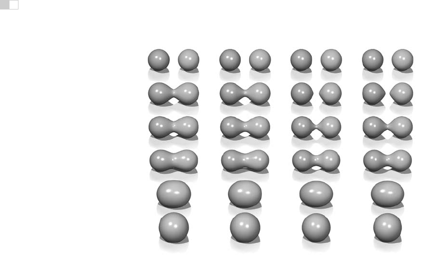
Figure 16.3. Each column shows two point primitives approaching each other. From left
to right: the fall-off filter functions used are Blobby, Metaball, soft objects, and Wyvill.
Image
courtesy Erwin DeGroot
.
where n skeletal elements contribute to the resulting field value. An example is
shown in (Figure 16.3) in which the field at any point (x, y, z) is calculated as in
Equation (16.3).
In this case, two point primitives are placed in close proximity. As the two
points are brought together, the surfaces bulge and then blend together. The term
filter function is used because the function causes the primitives to be blurred
together somewhat akin to a filter function for images. The summation blend is
the most compact and efficient blending operation that can be applied to implicit
surfaces (see Equation (16.3)).
One advantage of using filter functions with finite support is that primitives
that are far from p will have zero contribution and thus need not be consid-
ered (Wyvill et al., 1986).
16.1.1 C
1
Continuity and the Gradient
The most basic form of continuity is C
0
continuity, which ensures that there are no
“jumps” in a function. Higher-order continuity is defined in terms of derivatives
of functions (see Chapter 15).

i
i
i
i
i
i
i
i
16.1. Implicit Functions, Skeletal Primitives and Summation Blending 389
In the case of a 3D scalar field f,thefirst derivative is a vector function known
as the gradient, written ∇f and defined as
∇f(p)=
∂f(p)
∂x
,
∂f(p)
∂y
,
∂f(p)
∂z
.
If ∇f is defined at all points, and the three one-dimensional partial derivatives
are each C
0
,thenf is C
1
. Informally, C
1
surface continuity means that the
surface normal varies smoothly over the surface. The surface normal is the unit
vector perpendicular to the surface. If no unique surface normal can be defined
on the edge of a cube, for example, then the surface is not C
1
. For points on an
implicit surface the surface normal can be computed by normalizing the gradient
vector ∇f. In the example of the circle, points inside have a negative value and
those on the outside have a positive one. For many types of implicit surfaces, the
sense of inside and outside is inverted, and since the normal vector must always
point outwards, it can be opposite to the gradient direction.
Skeletal implicit primitives are created by applying a fall-off filter function to
an unsigned distance field as in Equation (16.2). Although the distance field is
never C
1
at the skeleton, these discontinuities can be removed by using a suitable
fall-off function (Akleman & Chen, 1999). If an operator, g, combines implicit
functions, f
1
and f
2
, where all points are C
1
,theng(f
1
,f
2
) is not necessarily
C
1
. For example it is possible to make a sharp CSG junction using the min and
max operators. The combination is not C
1
continuous because the min and max
operators don’t have that property (see Section 16.5).
The analysis of operators is complicated by the fact that it is sometimes de-
sirabletocreateaC
1
discontinuity. This case occurs whenever a crease in the
surface is desired. For example, a cube is not C
1
because tangent discontinu-
ities occur at each edge. To create creases using C
1
primitives, the operator must
introduce C
1
discontinuities, and hence cannot be C
1
itself.
16.1.2 Distance Fields, R-Functions, and F-Reps
The distance field is defined with respect to some geometric object T:
F(T, p)=min
q
∈T
|q − p|.
Visually, F(T, p) is the shortest distance from p to T. Hence, when p lies on T,
F(T, p)=0and the surface created by the implicit function is the object T.Out-
side of T, a non-zero distance is returned. The function T can be any geometric
entity embedded in 3D—a point, curve, surface, or solid. Procedural modeling
..................Content has been hidden....................
You can't read the all page of ebook, please click here login for view all page.