
i
i
i
i
i
i
i
i
354 15. Curves
Thus, the constraint matrix is
C =
⎡
⎢
⎢
⎣
1000
0100
1111
0123
⎤
⎥
⎥
⎦
,
and the basis matrix is
B = C
−1
=
⎡
⎢
⎢
⎣
1000
0100
−3 −23−1
21−21
⎤
⎥
⎥
⎦
.
We will discuss Hermite cubic splines in Section 15.5.2.
15.3.5 Blending Functions
If we know the basis matrix, B, we can multiply it by the parameter vector, u,to
get a vector of functions
b(u)=uB.
Notice that we denote this vector by b(u) to emphasize the fact that its value
depends on the free parameter u. We call the elements of b(u) the blending func-
tions, because they specify how to blend the values of the control point vector
together:
f(u)=
n
i=0
b
i
(u)p
i
. (15.11)
It is important to note that for a chosen value of u, Equation (15.11) is a linear
equation specifying a lin ear blend (or weighted average) of the control points.
This is true no matter what degree polynomials are “hidden” inside of the b
i
functions.
Blending functions provide a nice abstraction for describing curves. Any type
of curve can be represented as a linear combination of its control points, where
those weights are computed as some arbitrary functions of the free parameter.
15.3.6 Interpolating Polynomials
In general, a polynomial of degree n can interpolate a set of n +1values. If
we are given a vector p =(p
0
,...,p
n
) of points to interpolate and a vector

i
i
i
i
i
i
i
i
15.3. Polynomial Pieces 355
t =(t
0
,...,t
n
) of increasing parameter values, t
i
= t
j
, we can use the methods
described in the previous sections to determine an n +1×n +1basis matrix that
gives us a function f(t) such that f(t
i
)=p
i
. For any given vector t, we need to
set up and solve an n =1× n +1linear system. This provides us with a set of
n +1basis functions that perform interpolation:
f(t)=
n
i=0
p
i
b
i
(t).
These interpolating basis functions can be derived in other ways. One partic-
ularly elegant way to define them is the Lagrange form:
b
i
=
n
)
j=0,j=i
x − t
j
t
i
− t
j
. (15.12)
There are more computationally efficient ways to express the interpolating basis
functions than the Lagrange form (see De Boor (1978) for details).
Interpolating polynomials provide a mechanism for defining curves that in-
terpolate a set of points. Figure 15.3 shows some examples. While it is possible
to create a single polynomial to interpolate any number of points, we rarely use
high-order polynomials to represent curves in computer graphics. Instead, inter-
polating splines (piecewise polynomial functions) are preferred. Some reasons
for this are considered in Section 15.5.3.
1
2
3
4
5
1
2345
6
1
2
4
3
5
6
(a) Interpolating polynomial through (b) Interpolating polynomial through (c) Interpolating polynomial through five and six points
five points six points
Figure 15.3. Interpolating polynomials through multiple points. Notice the extra wiggles
and over-shooting between points. In (c), when the sixth point is added, it completely
changes the shape of the curve due to the non-local nature of interpolating polynomials.
i
i
i
i
i
i
i
i
356 15. Curves
15.4 Putting Pieces Together
Now that we’ve seen how to make individual pieces of polynomial curves, we can
consider how to put these pieces together.
15.4.1 Knots
The basic idea of a piecewise parametric function is that each piece is only used
over some parameter range. For example, if we want to define a function that
has two piecewise linear segments that connect three points (as shown in Fig-
ure 15.4(a)), we might define
f(u)=
f
1
(2u)if0≤ u<
1
2
,
f
2
(2u − 1) if
1
2
≤ u<1,
(15.13)
where f
1
and f
2
are functions for each of the two line segments. Notice that
we have re-scaled the parameter for each of the pieces to facilitate writing their
equations as
f
1
(u)=(1− u)p
1
+ up
2
.
For each polynomial in our piecewise function, there is a site (or parameter
value) where it starts and ends. Sites where a piece function begins or ends are
called knots. For the example in Equation (15.13), the values of the knots are
0, 0.5, and 1.
We may also write piecewise polynomial functions as the sum of basis func-
tions, each scaled by a coefficient. For example, we can re-write the two line
segments of Equation (15.13) as
f(u)=p
1
b
1
(u)+p
2
b
2
(u)+p
3
b
3
(u), (15.14)
0
.5
.5
1
0
.5
.5
1
b1(u)
b2(u)
b3(u)
p1
p2
p3
(a) (b)
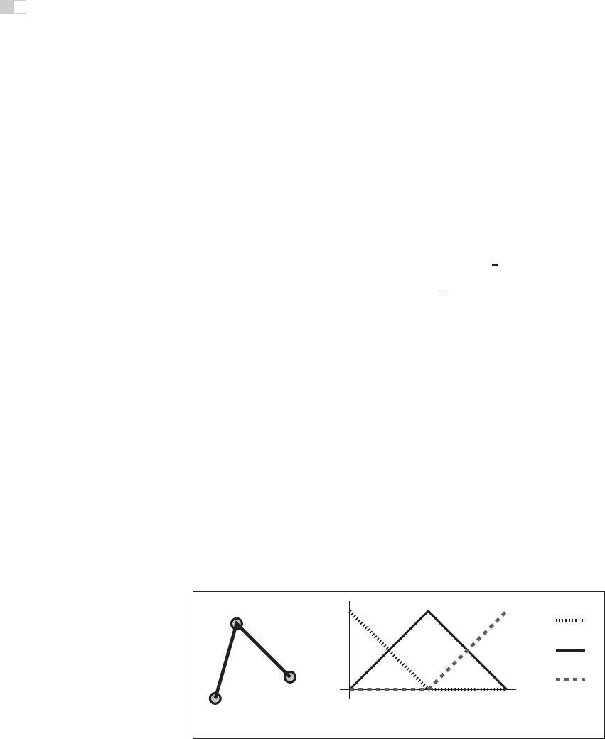
Figure 15.4. (a) Two line segments connect three points; (b) the blending functions for each
of the points are graphed at right.

i
i
i
i
i
i
i
i
15.4. Putting Pieces Together 357
where the function b
1
(u) is defined as
b
1
(u)=
1 − 2u if 0 ≤ u<
1
2
,
0otherwise,
and b
2
and b
3
are defined similarly. These functions are plotted in Figure 15.4(b).
The knots of a polynomial function are the combination of the knots of all of
the pieces that are used to create it. The knot vector is a vector that stores all of
the knot values in ascending order.
Notice that in this section we have used two different mechanisms for combin-
ing polynomial pieces: using independent polynomial pieces for different ranges
of the parameter and blending together piecewise polynomial functions.
15.4.2 Using Independent Pieces
In Section 15.3, we defined pieces of polynomials over the unit parameter range.
If we want to assemble these pieces, we need to convert from the parameter of the
overall function to the value of the parameter for the piece. The simplest way to
do this is to define the overall curve over the parameter range [0,n] where n is the
number of segments. Depending on the value of the parameter, we can shift it to
the required range.
15.4.3 Putting Segments Together
If we want to make a single curve from two line segments, we need to make sure
that the end of the first line segment is at the same location as the beginning of the
next. There are three ways to connect the two segments (in order of simplicity):
1. Represent the line segment as its two endpoints, and then use the same point
for both. We call this a shared-point scheme.
2. Copy the value of the end of the first segment to the beginning of the second
segment every time that the parameters of the first segment change. We call
this a dependency scheme.
3. Write an explicit equation for the connection, and enforce it through nu-
merical methods as the other parameters are changed.
While the simpler schemes are preferable since they require less work, they also
place more restrictions on the way the line segments are parameterized. For ex-
ample, if we want to use the center of the line segment as a parameter (so that the

i
i
i
i
i
i
i
i
358 15. Curves
user can specify it directly), we will use the beginning of each line segment and
the center of the line segment as their parameters. This will force us to use the
dependency scheme.
Notice that if we use a shared point or dependency scheme, the total number
of control points is less than n ∗ m, where n is the number of segments and m
is the number of control points for each segment; many of the control points of
the independent pieces will be computed as functions of other pieces. Notice
that if we use either the shared-point scheme for lines (each segment uses its two
Each line segment is parameterized by its endpoint and
its centerpoint.
Each line segment is parameterized by its endpoints.
The endpoint of segment two is equated
to the "free" end of segment one.
The end of one segment is shared with the beginning endpoint of the next segment.
Moving a control point causes a change only in a localized region.
A change in any control point causes
ALL later line segments to be affected.
The endpoint of segment three is equated
to the "free" end of segment two, etc.
Figure 15.5. A chain of line segments with local control and one with non-local control.
..................Content has been hidden....................
You can't read the all page of ebook, please click here login for view all page.