
i
i
i
i
i
i
i
i
612 23. Tone Reproduction
0.1
0.2
0.3
0.4
0.5
0.6
0.7
0.8
0.9
1.0
0.0
10 10 10 10 10 10 10 10
-3 -2 -1 0 1 2 3 4
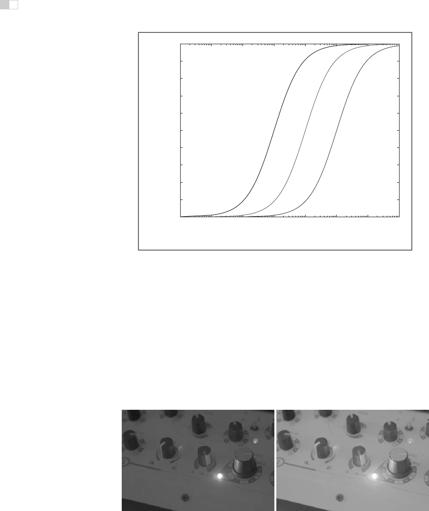
L = L / (L + 1)
dww
L = L / (L + 10)
dww
L = L / (L + 100)
dww
L
d
L
w
Figure 23.21. The choice of semi-saturation constant determines how input values are
mapped to display values.
The function f(x, y) may be computed in several different ways (Reinhard
et al., 2005). In its simplest form, f(x, y) is set to
¯
L
v
/k, so that the geometric
average is mapped to user parameter k (Figure 23.22) (Reinhard et al., 2002). In
this case, a good initial value for k is 0.18, although for particularly bright or dark
scenes this value may be raised or lowered. Its value may be estimated from the
image itself (Reinhard, 2003). The exponent n in Equation (23.3) may be set to 1.
In this approach, the semi-saturation constant is a function of the geometric
average, and the operator is therefore global. A variation of this global opera-
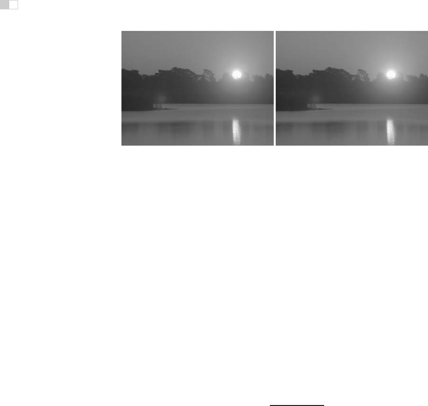
Figure 23.22. A linearly scaled image (left) and an image tonemapped using sigmoidal
compression (right).

i
i
i
i
i
i
i
i
23.9. Sigmoids 613
Figure 23.23. Linear interpolation varies contrast in the tonemapped image. The parameter
a
is set to 0.0 in the left image, and to 1.0 in the right image.
tor computes the semi-saturation constant by linearly interpolating between the
geometric average and each pixel’s luminance:
f(x, y)=aL
v
(x, y)+(1− a)
¯
L
v
.
The interpolation is governed by user parameter a which has the effect of vary-
ing the amount of contrast in the displayable image (Figure 23.23) (Reinhard &
Devlin, 2005). More contrast means less visible detail in the light and dark areas
and vice versa. This interpolation may be viewed as a half-way house between a
fully global and a fully local operator by interpolating between the two extremes
without resorting to expensive blurring operations.
Although operators typically compress luminance values, this particular op-
erator may be extended to include a simple form of chromatic adaptation. It thus
presents an opportunity to adjust the level of saturation normally associated with
tonemapping, as discussed at the beginning of this chapter.
Rather than compress the luminance channel only, sigmoidal compression is
applied to each of the three color channels:
I
r,d
(x, y)=
I
r
(x, y)
I
r
(x, y)+f
n
(x, y)
,
I
g,d
(x, y)=
I
g
(x, y)
I
g
(x, y)+f
n
(x, y)
,
I
b,d
(x, y)=
I
b
(x, y)
I
b
(x, y)+f
n
(x, y)
.
The computation of f(x, y) is also modified to bilinearly interpolate between the
geometric average luminance and pixel luminance and between each independent
color channel and the pixel’s luminance value. We therefore compute the geo-
metric average luminance value
¯
L
v
, as well as the geometric average of the red,
green and blue channels (
¯
I
r
,
¯
I
g
,and
¯
I
b
). From these values, we compute f(x, y)
i
i
i
i
i
i
i
i
614 23. Tone Reproduction
Figure 23.24. Linear interpolation for color correction. The parameter c is set to 0.0 in the
left image, and to 1.0 in the right image. (See also Plate XVII.)
for each pixel and for each color channel independently. We show the equation
for the red channel (f
r
(x, y)):
G
r
(x, y)=cI
r
(x, y)+(1− c) L
v
(x, y),
¯
G
r
(x, y)=c
¯
I
r
+(1− c)
¯
L
v
,
f
r
(x, y)=aG
r
(x, y)+(1− a)
¯
G
r
(x, y).
The interpolation parameter a steers the amount of contrast as before, and the new
interpolation parameter c allows a simple form of color correction (Figure 23.24
and Plate XVII).
So far we have not discussed the value of the exponent n in Equation (23.3).
Studies in electrophysiology report values between n =0.2 and n =0.9 (Hood et
al., 1979). While the exponent may be user-specified, for a wide variety of images
we may estimate a reasonable value from the geometric average luminance
¯
L
v
and
the minimum and maximum luminance in the image (L
min
and L
max
) with the
following empirical equation:
n =0.3+0.7
L
max
−
¯
L
v
L
max
− L
min
1.4
.
The several variants of sigmoidal compression shown so far are all global in na-
ture. This has the advantage that they are fast to compute, and they are very
suitable for medium to high dynamic range images. For very high dynamic range
images, it may be necessary to resort to a local operator, since this may give some
extra compression. A straightforward method to extend sigmoidal compression
replaces the global semi-saturation constant by a spatially varying function, which
may be computed in several different ways.
In other words, the function f(x, y) is so far assumed to be constant, but may
also be computed as a spatially localized average. Perhaps the simplest way to
i
i
i
i
i
i
i
i
23.9. Sigmoids 615
accomplish this is to once more use a Gaussian blurred image. Each pixel in
a blurred image represents a locally averaged value which may be viewed as a
suitable choice for the semi-saturation constant
1
.
As with division-based operators discussed in the previous section, we have
to consider haloing artifacts. However, when an image is divided by a Gaussian
blurred version of itself, the size of the Gaussian filter kernel needs to be large
in order to minimize halos. If sigmoids are used with a spatially variant semi-
saturation constant, the Gaussian filter kernel needs to be made small in order
to minimize artifacts. This is a significant improvement, since small amounts of
Gaussian blur may be efficiently computed directly in the spatial domain. In other
words, there is no need to resort to expensive Fourier transforms. In practice, filter
kernels of only a few pixels width are sufficient to suppress significant artifacts
while at the same time producing more local contrast in the tonemapped images.
One potential issue with Gaussian blur is that the filter blurs across sharp
contrast edges in the same way that it blurs small details. In practice, if there
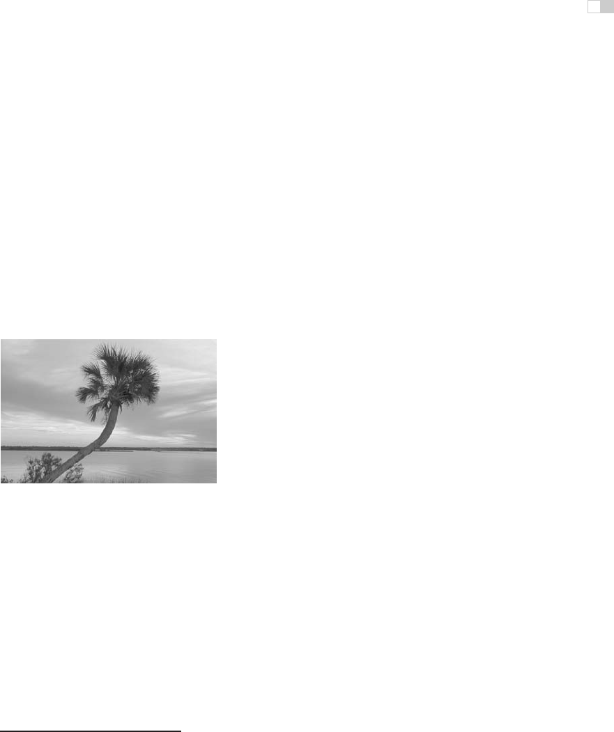
Figure 23.25. Example image used to
demonstrate the scale selection mechanism
shown in Figure 23.26.
is a large contrast gradient in the neigh-
borhood of the pixel under considera-
tion, this causes the Gaussian-blurred
pixel to be significantly different from
the pixel itself. This is the direct cause
for halos. By using a very large fil-
ter kernel in a division-based approach,
such large contrasts are averaged out.
In sigmoidal compression schemes,
a small Gaussian filter minimizes the
chances of overlapping with a sharp
contrast gradient. In that case, halos
still occur, but their size is such that they
usually go unnoticed and instead are perceived as enhancing contrast.
Another way to blur an image, while minimizing the negativeeffects of nearby
large contrast steps, is to avoid blurring over such edges. A simple, but compu-
tationally expensive way, is to compute a stack of Gaussian-blurred images with
different kernel sizes. For each pixel, we may choose the largest Gaussian that
does not overlap with a significant gradient.
In a relatively uniform neighborhood, the value of a Gaussian-blurred pixel
should be the same regardless of the filter kernel size. Thus, the difference be-
tween a pixel filtered with two different Gaussians should be approximately zero.
1
Although f(x, y) is now no longer a constant, we continue to refer to it as the semi-saturation
constant.

i
i
i
i
i
i
i
i
616 23. Tone Reproduction
Figure 23.26. Scale selection mechanism: the left image shows the scale selected for each
pixel of the image shown in Figure 23.25; the darker the pixel, the smaller the scale. A total
of eight different scales were used to compute this image. The right image shows the local
average computed for each pixel on the basis of the neighborhood selection mechanism.
This difference will only change significantly if the wider filter kernel overlaps
with a neighborhood containing a sharp contrast step, whereas the smaller filter
kernel does not.
It is possible, therefore, to find the largest neighborhood around a pixel that
does not contain sharp edges by examining differences of Gaussians at different
kernel sizes. For the image shown in Figure 23.25, the scale selected for each pixel
is shown in Figure 23.26 (left). Such a scale selection mechanism is employed by
the photographic tone reproduction operator (Reinhard et al., 2002) as well as in
Ashikhmin’s operator (Ashikhmin, 2002).
Once the appropriate neighborhood for each pixel is known, the Gaussian
blurred average L
blur
for this neighborhood (shown on the right of Figure 23.26)
may be used to steer the semi-saturation constant, such as for instance employed
by the photographic tone reproduction operator:
L
d
=
L
w
1. + L
blur
.
An alternative, and arguably better, approach is to employ edge-preserving
smoothing operators, which are designed specifically for removing small details
while keeping sharp contrasts in tact. Several such filters, such as the bilateral fil-
ter (Figure 23.27), trilateral filter, Susan filter, the LCIS algorithm and the mean
shift algorithm are suitable, although some of them are expensive to compute (Du-
rand & Dorsey, 2002; Choudhury & Tumblin, 2003; Pattanaik & Yee, 2002; Tum-
blin & Turk, 1999; Comaniciu & Meer, 2002).
23.10 Other Approaches
Although the previous sections together discuss most tone reproduction operators
to date, there are one or two operators that do not directly fit into the above cate-
..................Content has been hidden....................
You can't read the all page of ebook, please click here login for view all page.