

i
i
i
i
i
i
i
i
522 20. Light
Radiance is what we are usually computing in graphics programs. A won-
derful property of radiance is that it does not vary along a line in space. To see
why this is true, examine the two radiance detectors both looking at a surface
as shown in Figure 20.2. Assume the lines the detectors are looking along are
close enough together that the surface is emitting/reflecting light “the same” in
both of the areas being measured. Because the area of the surface being sampled
is proportional to squared distance, and because the light reaching the detector is
inversely proportional to squared distance, the two detectors should have the same
reading.
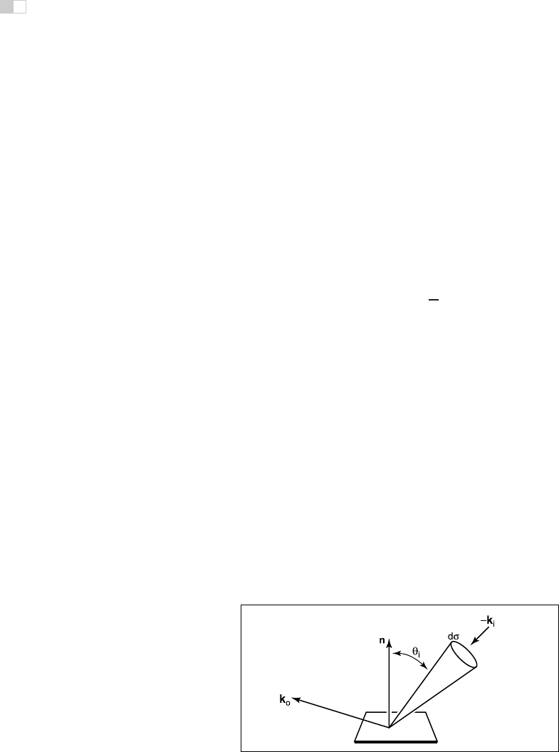
It is useful to measure the radiance hitting a surface. We can think of placing
the cone baffler from the radiance detector at a point on the surface and measur-
ing the irradiance H on the surface originating from directions within the cone
(Figure 20.3). Note that the surface “detector” is not aligned with the cone. For
this reason we need to add a cosine correction term to our definition of radiance:
response =
ΔH
Δσ cos θ
=
Δq
ΔA cos θ Δσ Δt Δλ
.
Figure 20.3. The ir-
radiance at the surface as
masked by the cone is
smaller than that measured
at the detector by a cosine
factor.
As with irradiance and radiant exitance, it is useful to distinguish between radi-
ance incident at a point on a surface and exitant from that point. Terms for these
concepts sometimes used in the graphics literature are surface radiance L
s
for
the radiance of (leaving) a surface, and field radiance L
f
for the radiance incident
at a surface. Both require the cosine term, because they both correspond to the
configuration in Figure 20.3:
L
s
=
ΔE
Δσ cos θ
L
f
=
ΔH
Δσ cos θ
.
Radiance and Other Radiometric Quantities
If we have a surface whose field radiance is L
f
, then we can derive all of the
other radiometric quantities from it. This is one reason radiance is considered the
“fundamental” radiometric quantity. For example, the irradiance can be expressed
as
H =
all k
L
f
(k)cosθdσ.
Figure 20.4. The direction
k has a differential solid an-
gle
d
σ associated with it.
This formula has several notational conventions that are common in graphics
that make such formulae opaque to readers not familiar with them (Figure 20.4).
First, k is an incident direction and can be thought of as a unit vector, a direction,

i
i
i
i
i
i
i
i
20.1. Radiometry 523
or a (θ, φ) pair in spherical coordinates with respect to the surface normal. The
direction has a differential solid angle dσ associated with it. The field radiance is
potentially different for every direction, so we write it as a function L(k).
As an example, we can compute the irradiance H at a surface that has con-
stant field radiance L
f
in all directions. To integrate, we use a classic spherical
coordinate system and recall that the differential solid angle is
dσ ≡ sin θdθdφ,
so the irradiance is
H =
2π
φ=0
π
2
θ=0
L
f
cos θ sin θdθdφ
= πL
f
.
This relation shows us our first occurrence of a potentially surprising constant π.
These factors of π occur frequently in radiometry and are an artifact of how we
chose to measure solid angles, i.e., the area of a unit sphere is a multiple of π
rather than a multiple of one.
Similarly, we can find the power hitting a surface by integrating the irradiance
across the surface area:
Φ=
all x
H(x)dA,
where x is a point on the surface, and dA is the differential area associated with
that point. Note that we don’t have special terms or symbols for incoming ver-
sus outgoing power. That distinction does not seem to come up enough to have
encouraged the distinction.
20.1.6 BRDF
Because we are interested in surface appearance, we would like to characterize
how a surface reflects light. At an intuitive level, for any incident light coming
from direction k
i
, there is some fraction scattered in a small solid angle near the
outgoing direction k
o
. There are many ways we could formalize such a concept,
and not surprisingly, the standard way to do so is inspired by building a simple
measurement device. Such a device is shown in Figure 20.5, where a small light
source is positioned in direction k
i
as seen from a point on a surface, and a detec-
tor is placed in direction k
o
. For every directional pair (k
i
, k
o
), we take a reading
with the detector.
Now we just have to decide how to measure the strength of the light source
and make our reflection function independent of this strength. For example, if we

i
i
i
i
i
i
i
i
524 20. Light
Figure 20.5. A simple measurement device for directional reflectance. The positions of light
and detector are moved to each possible pair of directions. Note that both k
i
and k
o
point
away from the surface to allow reciprocity.
replaced the light with a brighter light, we would not want to think of the surface
as reflecting light differently. We could place a radiance meter at the point being
illuminated to measure the light. However, for this to get an accurate reading that
would not depend on the Δσ of the detector, we would need the light to subtend a
solid angle bigger than Δσ. Unfortunately, the measurement taken by our roving
radiance detector in direction k
o
will also count light that comes from points
outside the new detector’s cone. So this does not seem like a practical solution.
Alternatively, we can place an irradiance meter at the point on the surface be-
ing measured. This will take a reading that does not depend strongly on subtleties
of the light source geometry. This suggests characterizing reflectance as a ratio:
ρ =
L
s
H
,
where this fraction ρ will vary with incident and exitant directions k
i
and k
o
, H
is the irradiance for light position k
i
,andL
s
is the surface radiance measured in
direction k
o
. If we take such a measurement for all direction pairs, we end up
with a 4D function ρ(k
i
, k
o
). This function is called the bidirectional reflectance
distribution function (BRDF). The BRDF is all we need to know to characterize
the directional properties of how a surface reflects light.
Directional Hemispherical Reflectance
Given a BRDF it is straightforward to ask “What fraction of incident light is
reflected?” However, the answer is not so easy; the fraction reflected depends on
the directional distribution of incoming light. For this reason, we typically only

i
i
i
i
i
i
i
i
20.1. Radiometry 525
set a fraction reflected for a fixed incident direction k
i
. This fraction is called the
directional hemispherical reflectance. This fraction, R(k
i
) is defined by
R(k
i
)=
power in all outgoing directions k
o
power in a beam from direction k
i
.
Note that this quantity is between zero and one for reasons of energy conservation.
If we allow the incident power Φ
i
tohitonasmallareaΔA, then the irradiance
is Φ
i
/ΔA. Also, the ratio of the incoming power is just the ratio of the radiance
exitance to irradiance:
R(k
i
)=
E
H
.
The radiance in a particular direction resulting from this power is by the definition
of BRDF:
L(k
o
)=Hρ(k
i
, k
o
)
=
Φ
i
ΔA
.
And from the definition of radiance, we also have
L(k
o
)=
ΔE
Δσ
o
cos θ
o
,
where E is the radiant exitance of the small patch in direction k
o
.Usingthese
two definitions for radiance we get
Hρ(k
i
, k
o
)=
ΔE
Δσ
o
cos θ
o
.
Rearranging terms, we get
ΔE
H
= ρ(k
i
, k
o
)Δσ
o
cos θ
o
.
This is just the small contribution to E/H that is reflected near the particular k
o
.
To find the total R(k
i
), we sum over all outgoing k
o
. In integral form this is
R(k
i
)=
all k
o
ρ(k
i
, k
o
)cosθ
o
dσ
o
.
Ideal Diffuse BRDF
An idealized diffuse surface is called Lambertian. Such surfaces are impossible in
nature for thermodynamic reasons, but mathematically they do conserve energy.
The Lambertian BRDF has ρ equal to a constant for all angles. This means the
i
i
i
i
i
i
i
i
526 20. Light
surface will have the same radiance for all viewing angles, and this radiance will
be proportional to the irradiance.
If we compute R(k
i
) for a a Lambertian surface with ρ = C we get
R(k
i
)=
all k
o
C cos θ
o
dσ
o
=
2π
φ
o
=0
π/2
θ
o
=0
k cos θ
o
sin θ
o
dθ
o
dφ
o
= πC.
Thus, for a perfectly reflecting Lambertian surface (R =1), we have ρ =1/π,
and for a Lambertian surface where R(k
i
)=r,wehave
ρ(k
i
, k
o
)=
r
π
.
This is another example where the use of a steradian for the solid angle determines
the normalizing constant and thus introduces factors of π.
20.2 Transport Equation
With the definition of BRDF, we can describe the radiance of a surface in terms of
the incoming radiance from all different directions. Because in computer graphics
we can use idealized mathematics that might be impractical to instantiate in the
lab, we can also write the BRDF in terms of radiance only. If we take a small part
of the light with solid angle Δσ
i
with radiance L
i
and “measure” the reflected
radiance in direction k
o
due to this small piece of the light, we can compute
a BRDF (Figure 20.6). The irradiance due to the small piece of light is H =
Figure 20.6. The geometry for the transport equation in its directional form.
..................Content has been hidden....................
You can't read the all page of ebook, please click here login for view all page.