5.1 NATURAL NUMBERS MULTIPLICATION
5.1.1 Introduction
The most basic multiplication algorithms for n-digit × m-digit B-ary natural numbers (shift and add algorithms) proceed in two phases:
- Digitwise partial products (n × m),
- Multioperand addition.
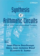
The classic computation scheme to introduce multiplication is given in Figure 5.1a, where partial products appear lined up according to their respective weight. This scheme is historically related to the pencil and paper implementation of the operation. This simple scheme is easily built up by noting that the partial products xi yj are lined up in the column whose index k = i + j corresponds to the weight Bk. Observe that whenever B > 2, the partial products may need two base-B digits. For B > 2, a possible multiplication scheme is displayed at Figure 5.1b, where XiYj and xiyj stand, respectively, for the integer product
and the mod B product
Observe that the column index k remains i + j for products (5.2) but is computed as i + j + 1 for products (5.1).
Figure 5.1 (a) Multiplication scheme and (b) multiplication scheme for B > 2.
The cost/speed constraints are key factors to set trade-offs between combinational parallel schemes and sequential implementations. The most popular algorithms, with a number of implementation schemes, are proposed in what follows, where n-digit by m-digit operands are considered for generality.
5.1.2 Shift and Add Algorithms
5.1.2.1 Shift and Add 1
Multiplication is known as a commutative operation in which both operands play the same mathematical role. At the algorithmic point of view, the situation is somewhat different. Actually, in most algorithm descriptions, one of the operands, called the multiplicator, is viewed as some kind of parameter set, while the other one, the multiplicand, is viewed as a data set.
Let the multiplicator X and the multiplicand Y be given by
![]()
Let
with
![]()
![]()
then
![]()
Equation (5.3) can be written
then expanded as
called the Hörner expansion. This suggests the following algorithm.1
Algorithm 5.1 Hörner Shift and Add 1
P(n):=0;
for i in 0..n-1 loop
     P(n-1-i):=P(n-i)*B+X(n-1-i)*Y;
end loop;
Z:=P(0);
5.1.2.2 Shift and Add 2
It will be shown in Chapter 12 that a right to left factorization (5.6) reduces by half the adder length.
Algorithm 5.2 Hörner Shift and Add 2
P(0):=0;
for i in 0..n-1 loop
     P(i+1):=(P(i)+X(i)*Y)/B;
end loop;
Z=P(n)*(B**n);
The difference between the roles of X and Y clearly appears in the recurrence formula of the Hörner Algorithms 5.1 and 5.2. At each step, the multiplicand Y is multiplied by X(k) then either (Algorithm 5.1) added to the (left-)shifted result of the preceding step or (Algorithm 5.2) added to the result of the preceding step and then (right-)shifted. The multiplicator component X(k) sets how many times the multiplicand Y has to be added. For B = 2, the process is quite simple because, at each step, X(k) ∈ {0,1} just sets if Y has to be added or not, while, whenever B ≥ 3, nontrivial partial products have to be generated.
Example 5.1 Let X = 367169 and Y = 24512 be two decimal numbers: n = 6, m = 5
The Hörner expressions (5.5) and (5.6) backing Algorithms 5.1 and 5.2 respectively, are:
![]()
and
![]()
Let us compute step by step.
Hörner Algorithm 5.1

Hörner Algorithm 5.2

This example illustrates the fact that in Algorithm 5.2, a digit is extracted at each step, so the complexity of the sum is always limited to n digits. In Algorithm 5.1, n + m digits are involved, and no digit is extracted before the end of the process. The same would occur in a standard addition process, whenever adding from left to right instead of right to left.
5.1.2.3 Extended Shift and Add Algorithm: XY + C + D
Observe that
![]()
in such a way that the full digit capacity of Z is not used, namely, n + m digits that would allow one to represent numbers up to (Bn+m −1). So, for the design of a device using this capacity, it is convenient to define the function
![]()
where C and D are n-digit and m-digit numbers, respectively, in such a way that
![]()
The modified Hörner Algorithm 5.2 is expressed as follows.
Algorithm 5.3 Extended Shift and Add
P(0):=D;
for i in 0..n−1 loop
     P(i+1):=(P(i)+X(i)*Y+C(i))/B;
end loop;
Z:=P(n)*(B**n);
Property 5.1 In the preceding algorithm, P(i) is an m + i number whose integer and fractional parts contain m and i digits, respectively
5.1.2.4 Cellular Shift and Add
Cellular Ripple-Carry Algorithm The recurrence operation of Algorithm 5.3 can be written in the form
![]()
where, according to Property 5.1,
![]()
so that
In what follows, p(i, j) stands for the jth digit of P(i). Expression (5.7) can be computed by an algorithm for adding natural numbers (basic addition Algorithm 4.1). Assuming that p(i, m + i − 1), …, p(i, 0) are the m + i digits of P(i), then the m + i + 1 digits p(i + 1, m + i), …, p(i + 1, 0) of P(i + 1) are computed as follows (symbol / stands for integer division):
Observe that p(i, i + j) ≤ B − 1 and xi.yj ≤ (B − 1)2, so that if carry(i, j) ≤ B − 1 then carry(i, j) + p(i, i + j) + xi. yj is a two-digit number (≤ B2 − 1), namely, [carry(i, j + 1), sum(i, j)] or carry(i, j + 1).B + sum(i, j). Thus an essential difference with the basic addition algorithm 4.1 (in base B > 2) comes from the range of the carry [0, B − 1] instead of [0, 1].
The precedence graph (Chapter 10) of the multiplication algorithm for n = 3, m = 4, is shown in Figure 5.2.
Algorithm 5.4 Cellular Ripple-Carry
(Symbol / stands for integer division)
for j in 0..m-1 loop p(0, j):=D(j); end loop,
for i in 0..n-1 loop
  carry(i, 0):=C(i);
  for j in 0..i-1 loop p(i+1, j):=p(i, j); end loop;
  for j in 0..m-1 loop
     p(i+1, i+j):=(p(i, i+j)+X(i)*Y(j)+carry(i, j)) mod B;
     carry(i, j+1):=(p(i, i+j)+X(i)*Y(j)+carry(i, j))/B;
  end loop;
  p(i+1, m+i):=carry(i, m);
end loop;
for j in 0..m+n-1 loop Z(j):=p(n, j); end loop;
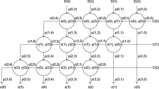
Figure 5.2 Ripple-carry multiplication algorithm–precedence graph (n = 3; m = 4).
Comment 5.1 The main loop, named (i, j)-cell loop, computes the functions carry(i, j + 1) and sum(i, j). The other loops are used for indexing purposes, such as assigning p(0, j) to D(j) or carry(i, 0) to C(i). The name cell takes its origin from the full-combinational cellular array implementation (Chapter 12, Section 12.2.3) of this algorithm. Actually, the (i, j)-cell can be implemented by any mix of hardware and firmware, where the choice can be made by the designer according to the resources at hand. As it will be shown in Chapter 12, the indexing is not trivial because the time performances can be directly and significantly affected. In a full-hardware implementation (Chapter 12), indexing p(i, j) corresponds to connection assignments between cells, as it already appears in Figure 5.2, where clear relationships come out between input and output indexes of (i, j)-cells.
Cellular Carry-Save Algorithm The following carry–save algorithm differs from the ripple-carry algorithm 5.4 by the indexing loops and a final adding stage loop. The basic concepts of carry-save adders (CSAs, Chapter 4) are applied in the way carries are saved from one loop to the other one, allowing more parallelism in the cell computation. The precedence graph of the carry-save multiplication algorithm for n = 3, m = 4, is shown in Figure 5.3.
Algorithm 5.5 Carry-Save
(Symbol / stands for integer division)
for j in 0..m-1 loop p(0, j):=D(j); carry(0, j):=C(j); end
loop;
for i in 0..n-2 loop p(i+1, m+i):=0; end loop;
for i in 0..n-1 loop
    for j in 0..i-1 loop p(i+1, j):=p(i, j); end loop;
    for j in 0..m-1 loop
      p(i+1, i+j):=(p(i, i+j)+X(i)*Y(j)+carry(i, j)) mod B;
      carry(i+1, j):=(p(i, i+j)+X(i)*Y(j)+carry(i, j))/B;
    end loop;
end loop;
for j in 0..n-1 loop Z(j):=p(n, j); end loop;
k(0):=0; p(n, n+m-1):=0;
for j in 0..m-1 loop
  Z(j+n):=(p(n, n+j)+c(n, j)+k(j)) mod B;
  k(j+1):=(p(n, n+j)+c(n, j)+k(j))/B;
end loop;

Figure 5.3 Carry-save multiplication algorithm-precedence graph (n = 3; m = 4).
Comment 5.2 The (i, j)-cell loop computation scheme of the carry-save algorithm is much the same as that of the ripple-carry one. But a final adding loop has to be executed. Nevertheless, thanks to the reindexing, significant time is saved by taking a better profit of parallelism, either in the software execution or in hardware implementation. In particular, a data-flow machine with m processing units could implement the program within n steps whose elementary time delay would be that of one (i, j)-cell. Despite their aspect, the precedence graphs of Figures 5.2 and 5.3 are not circuits, because no assumption is made about the way cells are implemented. Nevertheless, assuming a full combinational circuit implementation for such cells would convert those figures to explicit circuit schemes (Chapter 12).
Whenever B = 2, the practical implementation of the (i, j)-cell is quite simple, because the partial products xi.yj are expressed by a single bit while two B-ary digits are generally needed for higher base values.
Let us point out that the precedence graph of Figure 5.3 presents several 0 inputs. Therefore the related border cells may be accordingly simplified.
5.1.3 Long-Operand Algorithm
In the case of long-operand multiplications, it may be necessary to break down the n-digit (or m-digit) operands into s-digit slices. Assume that a procedure multiplier has been defined; it computes the product of two s-digit numbers (symbol / stands for integer division):
procedure multiplier (s: in natural; carry, w, x, y: in
digit_vector (0..s − 1); next_carry, z: out digit_vector
(0..s-1)) is
begin
  z:=(carry+w+x*y)mod(B**s);
  next_carry:=(carry+w+x*y)/(B**s);
end multiplier;
The procedure multiplier generates two s-digit numbers (≤ Bs − 1). The next algorithm computes the product Z = X.Y, where X is an n-digit number and Y is an m-digit one.
Algorithm 5.6 Long-Operand
for k in 0..s-1 loop zero(k):=0; end loop;
for j in 0..m/s-1 loop p(0, j):=zero; end loop;
for i in 0..n/s-1 loop
  carry(i, 0):=zero;
  for j in 0..m/s-1 loop
    multiplier(s, carry(i, j), p(i, i+j), X(i*s..i*s+s-1),
    Y(i*s..i*s+s-1), carry(i, j+1), sum(i, j));
  end loop;
    p(i+1, m/s+i):=carry(i, m);
    for j in 0..i-1 loop p(i+1, j):=p(i, j); end loop;
    for j in 0..m-1 loop p(i+1, j+i):=sum(i, j); end loop;
  end loop;
  for j in 0..m/s+n/s-1 loop Z(j*s..j*s+s - 1):=p(n, j);
  end loop;