6.3 CONVERGENCE (FUNCTIONAL ITERATION) ALGORITHMS

6.3.1 Introduction

Functional iteration algorithms represent division as a function. Numerical calculus techniques are used to solve, for example, Newton–Raphson equations or Taylor–MacLaurin expansions. These methods provide better than linear convergence, but the step complexity is somewhat more important than the one involved in digit recurrence algorithms. Since functional iteration algorithms use multiplication as a basic operation, the step complexity will mainly depend on the performance of the multiplication resources at hand ([FER1967], [FLY1970]). In practice, whenever the division process is integrated in a general-purpose arithmetic processor, one of the advantages comes from the availability of multiplication without additional hardware cost. It has been reported ([OBE1994], [FLY1997]) that, in typical floating-point applications, sharing multipliers does not significantly affect the overall performances of the arithmetic unit. In what follows, the divisor d is assumed to be a positive and normalized number such that, for example, 1/B ≤ d < 1. In most practical binary applications, IEEE normalization standards are used: 1 ≤ d < 2.

6.3.2 Newton–Raphson Iteration Technique

Coming back to the general division equation written

the theoretical exact quotient (r = 0) may be written

Actually, the Newton–Raphson method first computes the reciprocal x of the divisor d, with the required precision, and then the result is multiplied by the dividend D. Using x = 1/d as a root target, the priming function

may be considered for root extraction {x|f(x) = 0}. To solve f(x) = 0, the following equation is iteratively used to evaluate x:

where f′(x_i) stands for (df/dx)_i, that is, the first derivative of f(x) at point x_i.

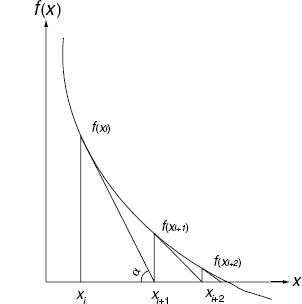
Figure 6.11 Newton–Raphson convergence graph.

The first steps of (6.61) are depicted in Figure 6.11. Equality (6.61) is readily inferred from

that points to x_i+1 as the intersection of the x-axis with the tangent to f(x) at x = x_i. Function (6.60) is continuous and derivable in the area (close enough to the root) where the successive approximations are processed. In base B, assuming d in [1/B, 1[, any value of x in ]1, B] could be chosen as a first approximation. To speed up the convergence process, a look-up table (LUT) is generally used for a first approximation. Let x₀ (≠ 0) be this first approximation; then

Using (6.61):

and recursively

In base 2, if d is initially set to

then

Selecting x₀ within the range 1 < x₀ ≤ 2 will ensure a quadratic convergence. Actually, assuming x_i = 1/d + ε_i, error ε_i+1 can be evaluated, according to (6.62), as

ending at

which means that, at each step, the number of relevant digits is multiplied by two. If x₀ is drawn from a t-digit precision LUT, the minimum precision p will be reached after k = log₂p/t steps.

Algorithm 6.11 Reciprocal Computation

x(0):=LUT (d);
for i in 0..k-1 loop
x(i+1):=x(i)*(2-d*x(i));
end loop;
Q:=x(k);

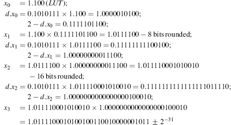
Example 6.8 Let d = 0.1618280 (base 10) and compute 1/d with precision 32.

Assume a look-up table with 4-digit precision.

In Example 6.8, one can observe that the error is always by default (as 2 − dx_i > 1). This is in agreement with the monotony of the convergence (Figure 6.11). Nevertheless, the practical convergence could appear different according to the way the rounding on the last digit is made: by excess or by default. Two dependent multiplications and one subtraction are needed at each computation step. In base B the subtraction can be substituted by (i) setting the integer part to 1 and (ii) a digitwise (B − 1)'s complement operation then (iii) adding 1 at the last digit level; the add-1 operation can be skipped to speed up the process at the cost of a slower convergence rate. In base 2 the subtraction is actually a 2's complement operation, which in turn can be replaced by a bitwise complementation at the cost of a slower convergence rate. Example 6.9 illustrates the algorithm in base 2.

Example 6.9 Let d = 0.1010111 in base 2; compute 1/d with precision 32.

Assume a look-up table with 4-digit (rounded) precision.

The same example is now treated replacing the 2's complement operation by bitwise complementation.

6.3.3 MacLaurin Expansion—Goldschmidt's Algorithm

Taylor expansions are well-known mathematical tools for the numerical calculus of functions. The MacLaurin series, as the Taylor expansion of the function 1/(1 + x), is the base of a division algorithm called Goldschmidt's algorithm ([GOL1964]).

Consider the classical Taylor expansion at point p

applied to the function

At the point x = 0, the following MacLaurin expansion is established:

or equivalently,

This is the foundation of Goldschmidt's algorithm. As the Newton–Raphson method does, the series expansion technique consists of computing the reciprocal 1/d of the divisor d. The series 1/(1 + x) at x = 0 is easier to compute than 1/x at x = 1. The problem at hand is now to let D/d converge toward Q/1, which is readily achieved through successive multiplications by the factors of MacLaurin expression (6.69).

For this purpose, the following is assumed:

The procedure is then carried out as follows:

d(0) and D(0) are set to d and D respectively; a look-up table evaluation procedure could refine this first approximation to get a better convergence rate. Then

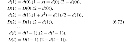
Algorithm 6.12 Goldschmidt's Algorithm

d(0):=LUT (divisor); DD(0):=LUT (dividend);
for i in 1..k-1 loop
d(i):=d(i-1)*(2-d(i-1));
DD(i):=DD(i-1)*(2-d(i-1));
end loop;
Q:=DD(k-1);

Comments 6.7

1. Each step is made up of one subtraction (2's complement in base 2) and two multiplications.
2. At step i, the computed value of d(i) is given by d(i) = 1 − x^exp(i) where exp(i) = 2ⁱ; since (6.70) 1/B ≤ d < 1, then (1 − B)/B ≤ x < 0, as initial pre-scaling of d and D is carried out, a fast quadratic convergence is ensured: each correction factor (1 + x^exp(i)) will duplicate the precision.
3. The complexity of the Newton–Raphson method is similar to the one involved in Goldschmidt's algorithm. Nevertheless, Goldschmidt's method directly provides the quotient while Newton–Raphson computes the reciprocal first, then a further multiplication is needed. Moreover, in Newton–Raphson, the two multiplications are dependent so they have to be processed sequentially while parallelism is allowed in Goldschmidt's method.
4. Newton Raphson's convergence method is self-correcting in the sense that any error (i.e., taking bitwise complement instead of 2's complement) is corrected in the following steps. On the contrary any error in Goldschmidt's algorithm will never be corrected. The final result will be the quotient of D(j)/d(j), assuming step j is the step where the last errors have been committed.
5. Goldschmidt's algorithm has been used in the IBM System/360 model 91 ([AND1967]) and, more recently, in the IBM System/390 ([SCHW1999]) and AMD-K7 microprocessor ([OBE1999]). Another algorithm based on series expansions has been implemented in IBM's Power3 ([SCHM1999]).
6. Goldschmidt's algorithm is suited for combinatorial implementations; factors of (6.72) can be calculated in parallel.

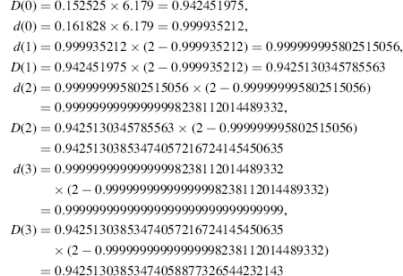
Example 6.10 Let D = 0.152525, d = 0.161828 (base 10); compute D/d with precision 32.

A look-up table with four-digit precision would approximate 1/d at 6.179, so multiplying both d and D by this value allows presetting d(0) and D(0) while reducing the number of steps:

Comment 6.8 An important question about convergence algorithms is the evaluation of the exact (i.e., minimum) amount of bits necessary for any prescaling or intermediate calculations, to ensure a correct result within the desired precision. Actually, the accurate calculus of rounding errors (LUT data as well as outputs from intermediate operations) is not a straightforward matter. This mathematical problem has been treated extensively in the literature ([DAS1995], [COR1999], [EVE2003]). Using extrabits is a safe and easy way to ensure correctness; nevertheless, a careful error computation can lead to significant savings ([EVE2003]).