
6.2 INTEGERS
6.2.1 General Algorithm
Let X be an integer and Y a natural number with Y > 0. Define Q and R respectively as the quotient and the remainder of the division of X by Y, with an accuracy of p fractional base-B digits:
![]()
where Q and R are integers, − Y ≤ R < Y and sign(R) = sign(X). In other words,
so that the unit in the least significant position (ulp) of Q.B−p and R.B−p is equal to B−p. In the particular case where p = 0, that is,
Q and R are the quotient and the remainder of the integer division of X by Y.
The basic algorithm applies to operands X and Y such that
In the general case, to ensure that −Y ≤ X < Y, a previous alignment step is necessary. Assume that X is an m-digit reduced B's complement number, that is, −Bm−1 ≤ X < Bm−1; then
substitute Y by Y′ = Bm−1.Y, so that Y′ ≥ Bm−1.1 > X and − Y′ ≤ − Bm−1.1 ≤ X; compute the quotient Q and the remainder R′ of the division of X by Y′, with an accuracy of p + m − 1 fractional base-B digits, that is,
![]()
that is,
![]()
Comment 6.2 If X is negative and X.Bp is an exact multiple of Y, for example, X.Bp = K.Y, then the remainder must be negative, so that
![]()
Nevertheless, the desired result was (probably)
![]()
An alternative definition of the quotient and remainder could be
![]()
that is, Definition 2.4.
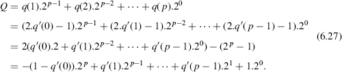
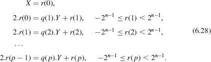
The digit-recurrence algorithms are based on the following sequence of equations:

Multiply the first equation by Bp, the second by Bp−1, the third by Bp−2, and so on. Then sum up the p + 1 equations. The following relation is obtained:
So
As a matter of fact, the 2-unknowns (q(i + 1), r(i + 1)) system
![]()
has two solutions as the interval − Y ≤ r(i + 1) < Y includes two values of r(i + 1) such that r(i + 1) ≡ B.r(i) mod Y. Thus different algorithms can be defined according to the way the values of r(i + 1) and q(i + 1) are chosen. The range of q(i + 1) is given by the following inequalities:
![]()
thus
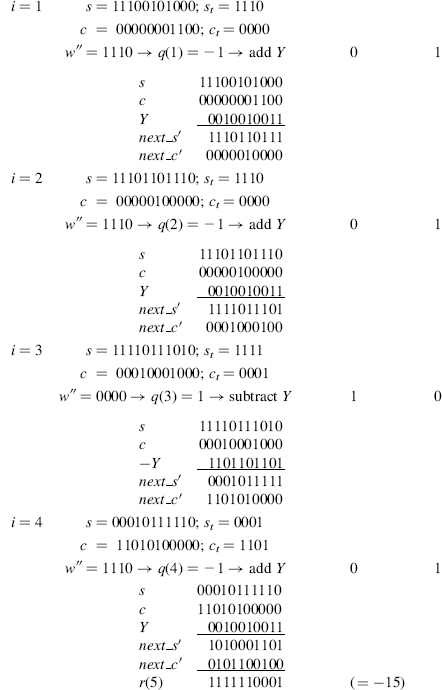
The diagram of Figure 6.1 (the Robertson diagram) gives, for every value of B.r(i), the two possible values of r(i + 1) along with the corresponding value of q(i + 1).
According to (6.25) the values of q(i) computed with (6.22) are not necessarily base-B digits. If the minimum and maximum values − B and B are not used, then q(i) is a signed base-B digit. An easy way to transform the obtained signed-digit representation into a nonsigned one (e.g., a B's complement representation) consists in defining, at each step, the ith component of two new variables q_pos and q_neg:

Figure 6.1 Robertson diagram: computation of r(i + 1) and q(i + 1).
- if q(i) > 0 then q_pos = q(i), q_neg = 0,
- if q(i) = 0 then q_pos = 0, q_neg = 0,
- if q(i) < 0 then q_pos = 0, q_neg = − q(i),
so that both q_pos and q_neg are p-digit base-B numbers. It remains to compute
![]()
As a matter of fact, the conversion from the signed-digit representation to a B's complement one can also be performed on the fly ([ERC1987], [ERC1992], [OBE1997]).
A final step is necessary in order that the condition sign(R) = sign(X) be satisfied:
if R < 0 and X ≥ 0 then substitute R by R + Y and Q by Q − 1;
if R ≥ 0 and X < 0 then substitute R by R − Y and Q by Q + 1.
Comment 6.3 If a previous alignment is necessary, instead of substituting Y by Y′ = Bm−1.Y, an alternative option is to substitute X by X′ = X/B and Y by Y′ = Bm−2.Y, and to compute the quotient Q and the remainder R′ of the division of X′ by Y′, with an accuracy of p + m − 1 fractional base-B digits, that is,
![]()
so that
![]()
Observe that the substitution of X by X′ is equivalent to the substitution of the first algorithm step, namely,
![]()

Figure 6.2 Restoring algorithm.
by
![]()
6.2.2 Restoring Division Algorithm
A simple way of choosing between the two possible values of r(i + 1) is to add the condition
![]()
so that all remainders have the same sign as X. Assume that X is nonnegative. Then the diagram of Figure 6.1 is reduced to the right upper quarter (Figure 6.2). The corresponding algorithm is the classical restoring algorithm of Section 6.1.
6.2.3 Base-2 Nonrestoring Division Algorithm
In the binary case, the diagram of Figure 6.1 (without the minimum and maximum values −2 and 2) is reduced to the diagram of Figure 6.3a. The way the values of r(i + 1) and q(i + 1) are chosen is shown in Figure 6.3b. The main difference with respect to the recovering algorithm is that the decision about the values of r(i + 1) and q(i + 1) only depends on the sign of r(i), and it is no longer necessary to compare 2.r(i) with Y:
- if 2.r(i) is nonnegative, then choose q(i + 1) = 1 and r(i + 1) = 2.r(i) − Y;
- if 2.r(i) is negative, then choose q(i + 1) = − 1 and r(i + 1) = 2.r(i) + Y.
The corresponding algorithm is the following:
Algorithm 6.5 Nonrestoring Division, First Version
r(0):=X;
for i in 0..p-1 loop
  if r(i)<0 then q_pos(i+1):=0; q_neg(i+1):=1;
  r(i+1):=2*r(i)+Y;
  else q_pos(i+1):=1; q_neg(i+1):=0; r(i+1):=2*r(i)-Y;
  end if;
end loop;
Q:=q_pos-q_neg;
R:=r(p);
if X>=0 and R<0 then R:=R+Y; Q:=Q-1;
elsif X<0 and R>=0 then R:=R-Y; Q:=Q+1;
end if;

Figure 6.3 Base-2 nonrestoring algorithm.
Nevertheless, a better algorithm, including an implicit on-the-fly conversion, can be used. At each step, instead of computing q(1), q(2), and so on, the following values are computed:
Observe that these new coefficients are bits:
- if q(i) = 1, then q′(i − 1) = 1;
- if q(i) = − 1, then q′(i − 1) = 0.
According to (6.24) and (6.26),
Thus the vector
![]()
is the 2's complement representation of Q.
The corresponding algorithm is the following:
Algorithm 6.6 Nonrestoring Division, Second Version
r(0):=X;
for i in 0..p-1 loop
  if r(i)<0 then Q(i):=0; r(i+1):=2*r(i)+Y;
  else Q(i):=1; r(i+1):=2*r(i)-Y;
  end if;
end loop;
Q(0):=1-Q(0); Q(p):=1; R:=r(p);
if X>=0 and R<0 then R:=R+Y; Q:=Q-1;
elsif X<0 and R>=0 then R:=R-Y; Q:=Q+1;
end if;
Observe that, before the final sign correction, the obtained quotient Q is always odd.
Examples 6.3
1. Compute − 12/15 with an accuracy of 8 fractional bits:

So Q = 100110011 = −205, R = 3, and 28.(−12) = (−205).15 + 3. The sign correction generates the final result: Q = (−205) +1 = −204, R = 3 − 15 = −12, so that 28.(−12) = (−204).15 + (−12).
2. (Integer division) Given a 9-bit integer X(−256 ≤ X < 256) and a positive integer Y, the integer division of X by Y is computed as follows. The divisor Y is substituted by Y′ = Y.256, the accuracy is equal to p + m − 1 = 0 + 9 − 1 = 8 bits, and the final remainder R′ will be substituted by R = R′/256. As an example, assume that X = −247 and Y = 15:
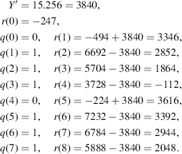
So, Q = 111101111 = −17, R = 2048/256 = 8, and −247 = (−17).15 + 8. The sign correction generates the final result: Q = (−17) + 1 = −16, R = 8 − 15 = − 7, so that −247 = (−16).15 + (−7).
The same operation can be performed taking into account Comment 6.3:

So, Q = 111101111 = −17, R = 1024/128 = 8, and −247 = (−17).15 + 8. The sign correction generates the final result: Q = (−17) + 1 = − 16, R = 8− 15 = − 7, so that −247 = (−16).15 + (−7).
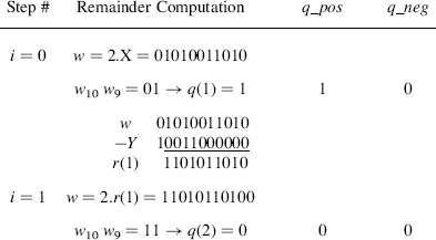
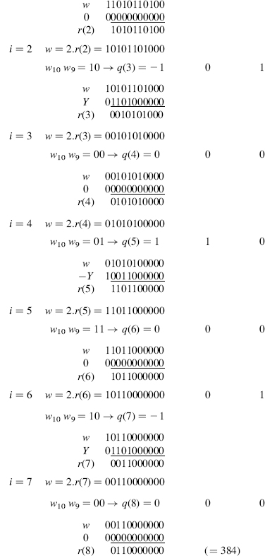
3. Given a 7-bit 2's complement integer X and a 6-bit natural number Y belonging to the interval −23.Y ≤ X < 23.Y, compute X/Y with an accuracy of p = 5. To ensure that − Y ≤ X < Y, the divisor is substituted by Y′ = 22.Y, the dividend by X′ = X/2, the division is performed with an accuracy of p = 5 + 3 = 8, and the final remainder will be divided by 22. Assume that X = 1010101 (−43) and Y = 000111 (7):
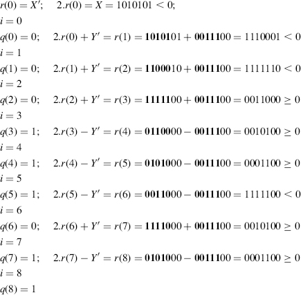
Thus Q = 100111011 and R = 0001100. Since X < 0 and r(8) > 0, a correction has to be made:
![]()
so that (−43).32 = (−196).7 + (−16/4), that is, −43 = (−196/32).7 + (−4/32).
Observe that Y′ is a multiple of 22, so that the operation 2.r(i) ± Y′ is performed with the five(boldface) most significant bits of 2.r(i) and Y′; the other bits of 2.r(i) are just propagated to the next step.
4. Given a 7-bit 2's complement integer X and a 6-bit natural number Y belonging to the interval − 24.Y ≤ X < 24.Y, compute X/Y with an accuracy of p = 4. To ensure that − Y ≤ X < Y, the divisor is substituted by Y′ = 23.Y, the dividend by X′ = X/2, the division is performed with an accuracy of p = 4 + 4 = 8, and the final remainder will be divided by 23. Assume that X = 00101011 (43) and Y = 000101 (5):
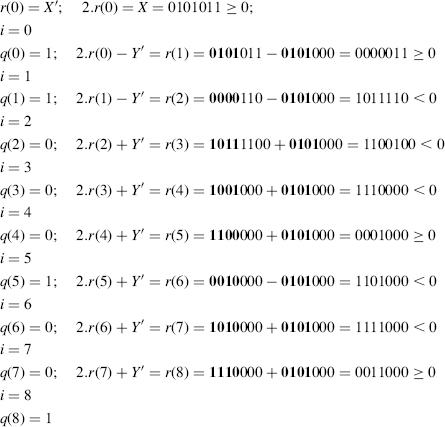
Thus Q = 010001001 ( = 137) and R = 0011000 ( = 24). Since X ≥ 0 and r(8) ≥ 0, no corrections have to be made, so that 43.16 = 137.5 + 24/23, that is, 43 = (137/16).5 + (3/16).
6.2.4 SRT Radix-2 Division
Consider again the diagram of Figure 6.3a. There are two overlapping areas such that
- if − Y ≤ 2.r(i)<0 then q(i + 1) can be chosen equal to either − 1 or 0;
- if 0 ≤ 2.r(i) < Y then q(i + 1) can be chosen equal to either 0 or 1.
The initial goal of the SRT-2 procedure was to reduce the number of additions or subtractions, choosing q(i + 1) = 0 and r(i + 1) = 2.r(i) as often as possible. Another advantage of the existence of overlapping areas is that, within particular conditions of allowed range on the remainder, the choice of q(i + 1) can be done as a function of the truncated values of Y and r(i). The drawback is the nonunique form of the final quotient because of the use of a redundant quotient-digit set, namely, {−1, 0, 1}. This is solved through a final conversion process.
If the strategy consists in selecting q(i + 1) = 0 whenever possible, the selection is achieved according to the following rule (Figure 6.3a):
- if 2.r(i) < − Y, then q(i + 1) = − 1;
- if − Y ≤ 2.r(i) < Y, then q(i + 1) = 0;
- if 2.r(i) ≥ Y, then q(i + 1) = 1.
In practice, detecting the situation that allows q(i + 1) = 0 (i.e., − Y ≤ 2.r(i) < Y) is not straightforward, unless through a trial subtraction, an operation to be avoided whenever possible to make the savings effective. Sweeney, Robertson, and Tocher ([SWE1957], [ROB1958], [TOC1958]) suggest an alternative solution to this question. Instead of allowing the range − Y ≤ r(i) < Y for the partial remainders, a restricted range is enforced.
Let Y be an n-bit natural number whose most significant bit is equal to 1, that is,
![]()
and X an integer belonging to the range
![]()
(an n-bit 2's complement number) so that − Y ≤ X < Y. Then the system (6.22), with B = 2, is substituted by the following:
The corresponding graphical representation is shown in Figure 6.4a.
The selection of q(i + 1) and r(i + 1) is done as follows (Figure 6.4b):
- if 2.r(i) < − 2n−1, then q(i + 1) = − 1, r(i + 1) = 2.r(i) + Y;
- if − 2n−1 ≤ 2.r(i) < 2n−1, then q(i + 1) = 0, r(i + 1) = 2.r(i);
- if 2.r(i) ≥ 2n−1, then q(i + 1) = 1, r(i + 1) = 2.r(i) − Y.
Observe that w = 2.r(i) belongs to the interval − 2n ≤ w < 2n. If it is represented as an (n + 1)-bit 2's complement number, the comparison with 2n−1 is very simple and can be done with the two most significant bits: See Table 6.1.
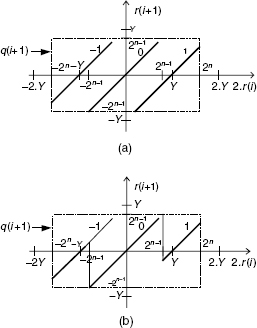
Figure 6.4 SRT-2 division algorithm.
The corresponding algorithm is the following:
Algorithm 6.7 SRT-2 Division
r(0):=X;
for i in 0..p-1 loop
  if 2.r(i)<-(2**(n-1))  then q_pos(i+1):=0; q_neg(i+1):=1;
  r(i+1):=2*r(i)+Y;
    elsif 2.r(i)>=2**(n-1)  then q_pos(i+1):=1; q_neg(i+1):=0;
    r(i+1):=2*r(i)-Y;
   else q_pos(i+1):=0; q_neg(i+1):=0; r(i+1):=2*r(i);
   end if;
end loop;
Q:=q_pos-q_neg;
R:=r(p);
if X>=0 and R<0 then R:=R+Y; Q:=Q-1;
elsif X<0 and R>=0 then R:=R-Y; Q:=Q+1;
end if;
TABLE 6.1 SRT-2 Algorithm: Selection of q(i + 1)
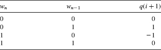
1. Given an 8-bit 2's complement integer X (−128 ≤ X < 128) and an 8-bit positive integer Y whose most significant bit is equal to 1 (128 ≤ Y < 256), compute the quotient and the remainder of the division of X by Y. The range of possible values of w is −256 ≤ w < 256. This range is partitioned into three intervals: w < −128, −128 ≤ w < 128 and 128 ≤ w, to which correspond the values −1, 0, and 1 for q(i + 1). Assume that X = − 84, Y = 247 and p = 8:
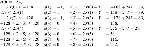
So q_pos = 01001000 ( = 72), q_neg = 10100000 ( = 160), Q = 72 − 160 = − 88, R = 232. The sign correction generates the final result: Q = (−88) + 1 = −87, R = 232 − 247 = −15, so that (−84).256 = (−87).247 + (−15).
2. Let X = 0101001101 ( = 333) be a 2's complement 10-bit integer and Y = 1101000000 ( = 832) a 10-bit natural number whose most significant bit is equal to 1. Compute X/Y with an accuracy of p = 8. At each step w will be represented in the form of a 2's complement number with 10 + 1 = 11 bits. For adding or subtracting Y, a 2's complement 11-bit representations will be used:
![]()
The step-by-step procedure is described as follows.
As the final remainder is positive, Y doesn't need to be added, and Q is given by:
![]()
The overall operation can be resumed as
![]()
6.2.5 SRT Radix-2 Division with Stored-Carry Encoding
The most time-consuming operation, at each step of algorithm 6.7, is clearly the computation of the new remainder r(i + 1): n-bit addition. The key idea for saving this time is to perform a carry-save sum, that is, a reduction of three operands to two (stored-carry encoding, Chapter 4). So every remainder r(i) will be expressed in the form of a sum of two 2's complement numbers. The SRT-2 carry-save algorithm departs from Algorithm 6.7 by the range allowed for the successive remainders and by the way the values of q(i + 1) and r(i + 1) are chosen as functions of r(i).
Let Y be an n-bit natural number whose most significant bit is equal to 1, that is,
and let X be an integer belonging to the range − Y ≤ X < Y, so that
![]()
(an (n + 1)-bit 2's complement number). Then the system (6.22), with B = 2, generates the quotient Q and the remainder R of the division of X by Y with an accuracy of p fractional bits. The selection of q(i + 1) and r(i + 1) must be done as shown in Figure 6.3a.
Every remainder r(i) belongs to the range − Y ≤ r(i) < Y, so that r(i) satisfies the following inequalities
![]()
and w = 2.r(i) belongs to the interval
In 2's complement, with n + 3 bits,
![]()
All along the algorithm execution, w will be represented in stored-carry form, that is, in the form
![]()
where s and c are (n + 3)-bit numbers (Figure 6.5a).

Figure 6.5 Stored-carry representation of w = 2.r(i).
Define w′ as being the truncated value of w = 2.r(j), namely (Figure 6.5b)
![]()
According to (6.30),
![]()
Thus
The maximum difference between w and w′.2n−1 is smaller than 2n−1, that is,
Define the truncated values st and ct of s and c as
![]()
and w″ as being the result of adding st and ct (Figure 6.5c). The difference between w′ and w″ is the possible carry from the rightmost positions, so that
that is, in 2's complement,
![]()
that is,
The selection of q(i + 1) is done as follows (see Figure 6.3a):
if − 5 ≤ w″ < − 1, that is, − 5 ≤ w″ ≤ − 2, then (6.36) w < 0 and q(i + 1) = −1;
if − 1 ≤ w″ < 0, that is, w″ = − 1, then (6.36) and (6.29) − Y ≤ − 2n−1 ≤ w < 2n−1 ≤ Y, and q(i + 1) = 0;
if 0 ≤ w″ ≤ 3, then (6.36) 0 ≤ w, and q(i + 1) = 1.
The corresponding selection rules are show in Table 6.2.
Assume that carry_save is a function that expresses the sum of three integers in the form of two integers (stored-carry encoding, Chapter 4). Then define an srt_step procedure:
procedure srt_step (s, c, Y: in integer; q_pos, q_neg: out
bit; next_s, next_c: out integer) is
begin
w″:=s(n+2..n-1)+c(n+2..n-1);
case w” is
  when 0000|0001|0010|0011|=>
    q_pos:=1; q_neg:=0; (next_s, next_c):=carry_save(s, c, -Y);
  when 1011|1100|1101|1110=>
    q_pos:=0; q_neg:=1; (next_s, next_c):=carry_save(s, c, Y);
  when others=>
    q_pos:=0; q_neg:=0; (next_s, next_c):=carry_save(s, c, 0);
  end case;
end srt_step;
The SRT-2 algorithm can now be stated as follows (s′ and c′ stand for s/2 and c/2):
Algorithm 6.8 SRT-2 Division with Stored-Carry Encoding
s′(0):=x; c′(0):=0;
for i in 0..p-1 loop
  srt_step(2*s′(i), 2*c′(i), y, q_pos(p-1-i), q_neg(p-1-i),
  s′(i+1), c′(i+1));
end loop;
r:=s′(p)+c′(p);
q:=q_pos-q_neg;
if x>=0 and r<0 then r:=r+y; q:=q-1;
elsif x<0 and r>=0 then r:=r-y; q:=q+1;
end if;
TABLE 6.2 SRT-2 Algorithm with Stored-Carry Encoding: Selection of q(i + 1)
| w″ | q(i + 1) |
| 0000 | 1 |
| 0001 | 1 |
| 0010 | 1 |
| 0011 | 1 |
| 0100 | — |
| 0101 | — |
| 0110 | — |
| 0111 | — |
| 1000 | — |
| 1001 | — |
| 1010 | — |
| 1011 | − 1 |
| 1100 | − 1 |
| 1101 | − 1 |
| 1110 | − 1 |
| 1111 | 0 |
Comment 6.4 When X belongs to the interval − Y ≤ X < 2n−1, it has been observed ([SUT2004]) that w″ never reaches 3, that is, −5 ≤ w″ ≤ 2. Then Table 6.2 can be modified as shown Table 6.3.
The most significant bit of w″, that is, ![]() , is no longer necessary and Table 6.3 is reduced Table 6.4.
, is no longer necessary and Table 6.3 is reduced Table 6.4.
TABLE 6.3 Modified q(i + 1) Selection Table
| w″ | q(i+1) |
| 0000 | 1 |
| 0001 | 1 |
| 0010 | 1 |
| 0011 | — |
| 0100 | — |
| 0101 | — |
| 0110 | — |
| 0111 | — |
| 1000 | — |
| 1001 | — |
| 1010 | — |
| 1011 | −1 |
| 1100 | −1 |
| 1101 | −1 |
| 1110 | −1 |
| 1111 | 0 |
TABLE 6.4 Reduced q(i + 1) Selection Table
| q(i + 1) | |
| 000 | 1 |
| 001 | 1 |
| 010 | 1 |
| 011 | −1 |
| 100 | −1 |
| 101 | −1 |
| 110 | −1 |
| 111 | 0 |
Examples 6.5
1. Let X = 001110111011 (=955) be a 12-bit 2's complement integer and Y = 11010101101 (=1709) an 11-bit positive integer. Compute X/Y with an accuracy of p = 8. At each step s and c will be represented in the form of 2's complement integers with 11 + 3 = 14 bits. For adding or subtracting Y, 2's complement 13-bit representations will be used:
![]()
The step-by-step procedure is described as follows (nop stands for no operation):

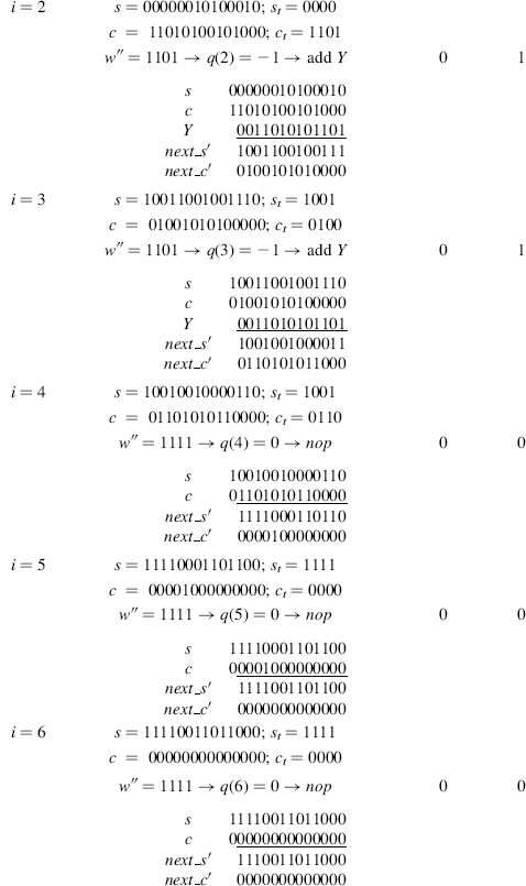
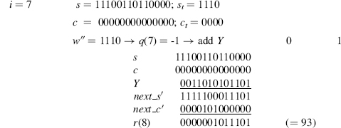
As the final remainder is positive, the divisor Y doesn't need to be added to the final remainder r(8), and Q is given by
![]()
In 2's complement:
![]()
The overall operation can be resumed as
![]()
2. Let Y be an 8-bit positive integer whose most significant bit is equal to 1 (128 ≤ Y < 256) and let X be a 9-bit 2's complement integer (−256 ≤ X < 255). In order to compute the X/Y with an accuracy of 4 fractional bits, X is first divided by 2 (Comment 6.3) and the division is performed with an accuracy of 5 fractional bits. Assume that X = 100000111 (−249) and Y = 10010011 (147). At each step s and c will be represented in the form of 2's complement integers with 8 + 3 = 11 bits. For adding or subtracting Y, 2's complement 10-bit representations will be used:
![]()
The step-by-step procedure is described as follows (nop stands for no operation):
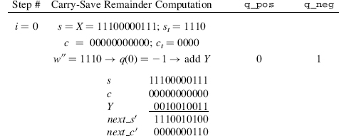
As the final remainder is negative, the divisor Y doesn't need to be subtracted from the final remainder r(5), and Q is given by
![]()
![]()
The overall operation can be resumed as
![]()
that is,
![]()
6.2.6 P–D Diagram
Apart from the Robertson diagram, another popular graphical tool used to illustrate the quotient selection problem is the P–D (partial remainder–divisor) plot diagram ([FRE1961]). It is a representation of the domain where possible values of the quotient-digit may be assigned. First define normalized values of Y, r(i), r(i + 1), w, w′, and w″:
so that
and the normalized values of w′ and w″ are
Thus
With these normalized values, the selection of q = q(i + 1) corresponding to Algorithm 6.8 (SRT division with stored-carry encoding) is done as follows (Figure 6.6):
if ![]() , then q = − 1.
, then q = − 1.
if ![]() , then q = 0;
, then q = 0;
if ![]() , q = 1.
, q = 1.
In the P−D diagram, the coordinates (2.r, d) are linked to none, one, or several acceptable values of q. Figure 6.7 displays the P−D diagram associated to the partial remainder diagram of Figure 6.6. The domain presented in Figure 6.7 covers the (2.r, d) coordinates compatible with the conditions ![]() ≤ d < 1 and − 2d ≤ 2.r < 2.d. This domain is divided into six zones separated by the lines 2.r = − 2.d, 2.r = − d, 2.r = 0, 2.r = d, and 2.r = 2.d. Above the line 2.r = 2.d and under the line 2.r = − 2.d lie two never reached zones; they correspond to coordinates out of range. Between the lines 2.r = − 2.d and 2.r = − d, the value −1 has to be assigned to q; this zone corresponds to the coordinates 2.r in the interval [− 2.d, − d[ of the diagram in Figure 6.6. Between the lines 2.r = − d and 2.r = 0, either value −1 or 0 may be assigned to q; this zone corresponds to the coordinates 2.r in the interval [− d, 0[ of the diagram in Figure 6.6. In the same way, one can show that in the positive field, the zone between the lines 2.r = 0 and 2.r = d corresponds to q in {0,1}, while the zone between the lines 2.r = d and 2.r = 2.d correspond to q = 1.
≤ d < 1 and − 2d ≤ 2.r < 2.d. This domain is divided into six zones separated by the lines 2.r = − 2.d, 2.r = − d, 2.r = 0, 2.r = d, and 2.r = 2.d. Above the line 2.r = 2.d and under the line 2.r = − 2.d lie two never reached zones; they correspond to coordinates out of range. Between the lines 2.r = − 2.d and 2.r = − d, the value −1 has to be assigned to q; this zone corresponds to the coordinates 2.r in the interval [− 2.d, − d[ of the diagram in Figure 6.6. Between the lines 2.r = − d and 2.r = 0, either value −1 or 0 may be assigned to q; this zone corresponds to the coordinates 2.r in the interval [− d, 0[ of the diagram in Figure 6.6. In the same way, one can show that in the positive field, the zone between the lines 2.r = 0 and 2.r = d corresponds to q in {0,1}, while the zone between the lines 2.r = d and 2.r = 2.d correspond to q = 1.
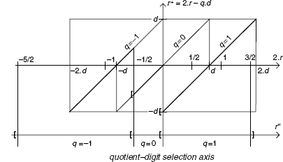
Figure 6.6 Robertson diagram.
Now the q selection strategy, defined in Figure 6.6, can be mapped on the P−D plot diagram: the lines r″ = − ![]() and r″ = 0, highlighted in Figure 6.7, set the limits for choosing q = −1, 0, or 1. As it appears in the following section, the P−D plot diagram is particularly well suited to deal with high-radix (bases 2k with k ≥ 2) because of more complex quotient-digit selection rules.
and r″ = 0, highlighted in Figure 6.7, set the limits for choosing q = −1, 0, or 1. As it appears in the following section, the P−D plot diagram is particularly well suited to deal with high-radix (bases 2k with k ≥ 2) because of more complex quotient-digit selection rules.
Actually, the P−D plot diagram as shown in Figure 6.7 is the level zero of a tri-dimensional (3-D) diagram whose third (vertical) axis would be r+, assuming that the horizontal axes are 2.r and d. Equations r+ = 2.r − q.d for q = −1,0, and 1 now represent planes crossing level zero at lines 2.r = −d, 2.r = 0, and 2.r = d, respectively. The diagram of Figure 6.6 is the intersection, at some allowed coordinate of d, of this tridimensional figure with a plane parallel to axes r+, 2.r, that is, parallel to plane d = 0. Figure 6.8 shows the 3-D Robertson/P–D diagram for the plane corresponding to q = −1. Lines 2.r = −d, 2.r = 0, and 2.r = d (from P–D plot diagram at r+ = 0) are highlighted in Figure 6.8, together with line r+ = 2.r − q.d (from the Robertson diagram at ![]() ).
).
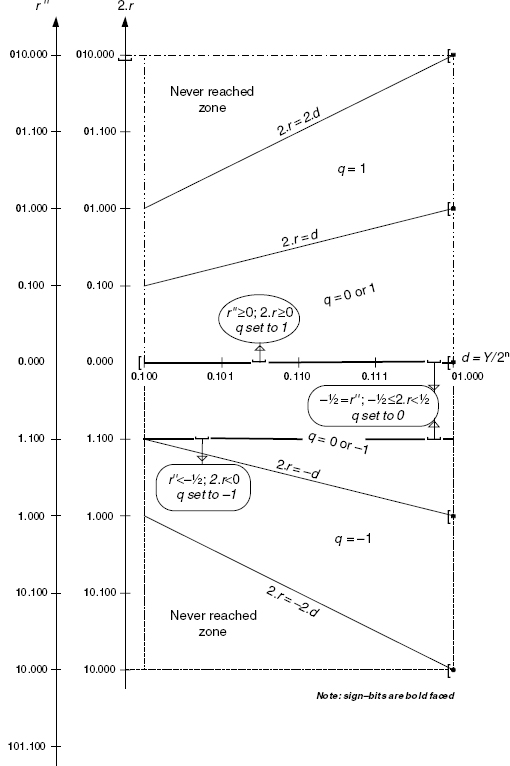
Figure 6.7 P−D plot diagram.

Figure 6.8 Tridimensional Robertson/P−D diagram for q = −1.
6.2.7 SRT-4 Division
The SRT method can be extended to any base 2k with a variety of quotient-digit sets. Nevertheless, the step complexity increases with k as more comparisons are involved in the quotient-digit selection process and more divisor multiples have to be computed. The designer will consider trade-offs between cycle time and the number of cycles. A lot of alternatives are proposed in the literature ([ERC1990], [ERC2004], [FAN1989], [MON1994], [QUA1992], [SRI1995], [TAY1985]). An SRT-4 (B = 22) algorithm, with redundant quotient-digit sets, is presented in the following.
One assumes that X and Y are n-bit 2's complement integers with

Figure 6.9 SRT-4 partial remainder diagram.
A first version is given with the quotient-digit set [− 3, 3]. This means that the multiples ± 2.Y and ± 3.Y have to be generated according to the possible selection of q = q(i + 1) = ± 2 or ± 3. The Robertson diagram is given in Figure 6.9.
The new remainder r(i + 1) is now computed as 4.r(i) − q(i + 1).Y, where q(i + 1) is selected in such a way that r(i + 1) can be kept in the range [−Y, Y[; the maximum allowed range for 4.r(i) is now [−2n+1, 2n+1[. As it will appear later, it is no longer possible to locate a point (4.r(i), Y) in some zone [k.Y, (k + 1).Y] of Figure 6.9, only from the numerical value 4.r(i). One also needs extra information on Y. The P−D plot diagram presented in Figure 6.10 emphasizes this point and illustrates a possible quotient-digit selection strategy (r stands for r(i) and q for q(i + 1)). Although the q-select zones are symmetric with respect to the Y-axis, the way to select q is not. This comes from the fact that, in 2's complement representation, truncated nonsign bits are always positive whatever the sign is. As in Figure 6.7, lines 4.r = q.Y are defining q-select zones. From Figure 6.9 one can check that between the vertical lines 4.r = k.Y and 4.r = (k + 1).Y, q can be either k or k + 1; this does not hold for the outermost zones where q has to be −3 or 3, according to the side; these zones are shown in Figure 6.10.
In Figure 6.10, the values on axis 4.r and Y have been truncated by n − 2 and n − 4 bits, respectively. For clarity, sign-bits appear as bold characters. The remaining bits are actually the only ones needed for algorithmic purposes. The q-selection strategy is illustrated in Figure 6.10 where heavy lines stand for border limit lines between consecutive options for q. The symbols “number & arrows” and “[”, lying on a border-line, respectively, highlight the choice for q, the zone covered by this choice, and the inclusion of the limit line in that choice. At coordinates 4.r = 010, 01, 11, and 10, horizontal border-lines still hold between regions of different options for q. This is no longer valid for values between [100, 101,[ and 011, 0100[, where so-called staircase lines emphasize that the selection in that case depends on Y too. Take a closer look at those border-lines to make sure that the selections proposed in Figure 6.10 are correct. First, remember that the bits deleted are always positive, so the head bits of 4.r or Y (truncated coordinates 4.r, Y) stand for the minimum of the nonintegers 4.r/2n−2 and Y/2n−4; notice that the rightmost point of any border-line is never reached as Y never reaches 01000. For these two reasons, the border-lines labeled −2, −1, 0, 1, and 2, in Figure 6.10, may include all the edge line points in the choice for q, extremities and corners included. The situation of the line labeled 3 is somewhat different: the choice q = 3 for the point labeled p1 is valid because p1 stands between two zones where this choice is allowed. The same principle holds for point p4 that moreover is never reached because of the above-mentioned limit condition on Y. Points p2 and p3 appear more critical as they are corner points in between border-lines with different choices. p3 = 3 is valid for standing inside a zone where this choice is allowed. p2 has to be excluded from the choice q = 3 (line p1 → p2) because, with full coordinates, this point could fall either in the zone q ∈ {1,2} or in the zone q ∈ {2,3}; thus p2 is given the value 2 of line p2 → p3.
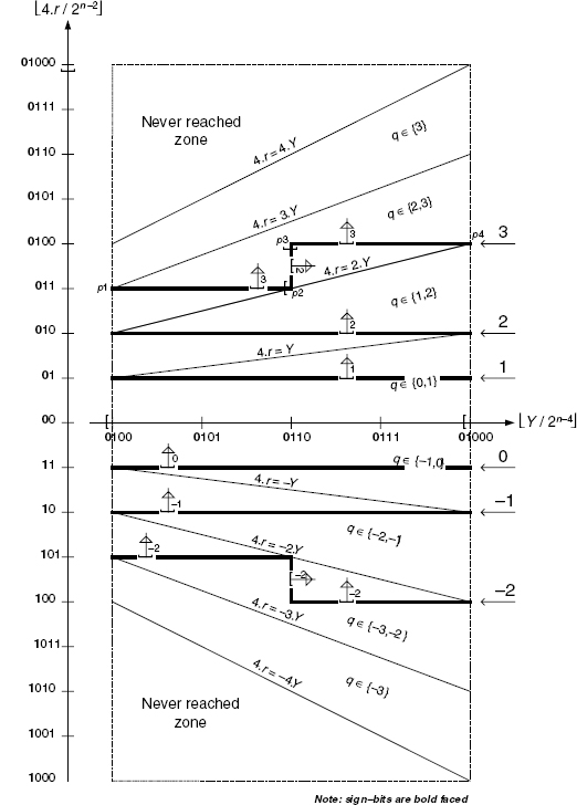
Figure 6.10 P−D plot diagram for SRT-4 division.
TABLE 6.5 SRT-4 Quotient-Digit Selection Table

The complete selection process can be resumed in Table 6.5.
Comment 6.5 For the sake of simplicity the truncated part of the exact n-bit remainder r(i) has been considered as coordinate references on Figure 6.10; four bits of the shifted remainder are required by the SRT-4 division algorithm 6.9. The carry-save techniques are applicable in this case, as far as a sufficient quantity of bits are saved in the st, ct representation of the remainder; moreover, the flexibility in the choice of the quotient-digit set, as well as that of the q-selection strategy, allows one to consider a number of alternatives in the algorithms. As in the SRT-2 case, the carry-save computation still has to be implemented in a way that prevents each of the carry-save components s′ and c′ from exceeding the (n + 2)-bit length.
Algorithm 6.9 SRT-4 Division
(/ Stands for integer division)
yt:=y/2**n-4
r(0):=X
for i in 0..p-1 loop
4.rt(i):=4.r(i)/2**n-2
if 4.rt(i)<-4 then q(i+1):=-3; q_pos(i+1):=0; q_neg
  (i+1):=3; r(i+1):=4.r(i)+3*Y;
elsif 4.rt(i)<-3 then
     if yt<6 then q(i+1):=-3; q_pos(i+1):=0; q_neg(i+1):=3;
     r(i+1):=4.r(i)+3*Y; else q(i+1):=-2; q_pos(i+1):=0;
  q_neg(i+1):=2; r(i+1):=4.r(i)+2*Y; end if;
elsif 4.rt(i)<-2 then q(i+1):=-2; q_pos(i+1):=0;
  q_neg(i+1):=2; r(i+1):=4.r(i)+2*Y;
elsif 4.rt(i)<-1 then q(i+1):=-1; q_pos(i+1):=0;
  q_neg(i+1):=1; r(i+1):=4.r(i)+Y;
elsif 4.rt(i)<1 then q(i+1):=0; q_pos(i+1):=0;
  q_neg(i+1):=0; r(i+1):=4.r(i);
elsif 4.rt(i)<2 then q(i+1):=1; q_pos(i+1):=1;
  q_neg(i+1):=0; r(i+1):=4.r(i)-Y;
elsif 4.rt(i)<3 then q(i+1):=2; q_pos(i+1):=2;
  q_neg(i+1):=0; r(i+1):=4.r(i)-2*Y;
elsif 4.rt(i)<4 then
if yt>=6 then q(i+1):=2; q_pos(i+1):=2; q_neg(i+1):=0;
     r(i+1):=4.r(i)-2*Y; else q(i+1):=3; q_pos(i+1):=0;
     q_neg(i+1):=3; r(i+1):=4.r(i)+3*Y; end if;
  else q(i+1):=3; q_pos(i+1):=0; q_neg(i+1):=3;
   r(i+1):=4.r(i)+3*Y; end if;
end loop;
q:=q_pos - q_neg;
If r(p)>=0 then R:=r(p); else R:=r(p)+Y; q:=q-1;
Example 6.6 Let X = 010110111100101100110 and Y = 011010110 be 2's complement numbers Compute X/Y with an accuracy of p = 6.
According to the conditions X in [−Y, Y[, and 2n−2 ≤ Y < 2n−1, a first preliminary scaling of Y is necessary: Y = 011010110000000000000. So, p = 6 + 12 = 18, n = 21, and two more bits will be necessary to express the multiples of Y.
First compute the multiples of Y as follows

For q-selection purposes one has to compute the integer division
![]()
The step-by-step procedure is described as follows (sign-bits are bold face; nop stands for no operation; symbol/stands for integer division).

As r(9) < 0, Y has to be added to the final remainder,
and the quotient has to be reduced by one unit. This can be done by reducing q_pos(8) to 1.
So the final quotient is given by
![]()
that is,
Q = (3, 2, 0, 0, 0, 2, 0, 0, 1) − (0, 0, 1, 0, 2, 0, 0, 2, 0,) = (3, 1, 2, 3, 2, 1, 3, 2, 1).
In binary, Q = 0110110111001111001, and the overall operation (accuracy 18 and pre-scaling 12) can be resumed as
![]()
Comment 6.6 As far as the final computation time for Q = Q_pos − Q_neg may be considered negligible with respect to the whole process, it may not be necessary to speed up the final conversion process. The influence of the conversion on the overall time will mainly depend on the required accuracy and the size of operands. On the other hand, the final correction on the last remainder, whenever negative, may be processed in parallel with the conversion process. To minimize the impact of the conversion time, several on-the-fly conversion algorithms have been proposed in the literature ([ERC1987], [ERC1992], [OBE1997]). Basically these algorithms perform the conversion as the digits are produced. Prescaling the divisor or both operands is another idea proposed in the literature ([ERC1983], [SVO1963]); as far as an efficient method can be used to make the divisor close enough to 1, the quotient-digit selection depends on the dividend only. As time has to be consumed for the scaling operation, the advantages are not clear in general cases. The SRT-4 algorithm has been used in the early Pentium processors and was the origin of the famous Pentium bug; the error, due to flaws in the look-up tables, was not detected on the test bench because the probability of addressing the tables at those incorrect entries was actually very weak ([EDE1997]).
6.2.8 Base-B Nonrestoring Division Algorithm
In bases other than 2 or 2k (high-radix), nonrestoring division algorithms have received little attention in the literature. Nevertheless, for the sake of generality, a more general approach on division algorithms with extended quotient-digit sets will be developed in the following.
Definitions 6.1
- A system of digits (weights) {di} is said to be complete when it is able to represent any number as a weighted sum of powers of the base B; a nonredundant quotient-digit system in base B is defined as a complete system of exactly B digits, that is, the minimum quantity of needed digit values to express the quotient (or any number) as a base-B number. The set {0, 1, …, B − 1} is most commonly used.
- In a redundant quotient-digit set, the number of allowed quotient-digits is greater than B. The most used sets are of the form {−α, −α +1, …, 0, …, α − 1, α} with α ≥
 B/2
B/2 , that is, a symmetric set of consecutive integers.
 - The redundancy factor ρ is defined as ρ = α/(B − 1).
- A quotient-digit set with α = B/2 is said to be minimally redundant.
- A quotient-digit set with α = B − 1(ρ = 1) is said to be maximally redundant.
- A quotient-digit set with α > B − 1 (ρ > 1) is said to be over-redundant.
The first algorithm to be presented for base-B nonrestoring division uses a redundant quotient-digit set {0, 1, 2, …, B}. A tentative quotient estimation is made from the truncated operands-look-up tables (LUTs) can be used to speed up this phase–then a possible correction has to be carried out in order to convert the obtained quotient into a final nonredundant representation. The following lemmas and theorems justify the algorithm.
Lemmas 6.2 Let
be two base-B positive integers (B ≥ 3, n ≥ 3). B.R, the shifted remainder, and Y, the divisor, comply with the following conditions:
Define moreover
Lemma 6.2.1
Proof The inequalities 0 ≤ qt and ![]() , are trivial.
, are trivial.
Condition (6.43) can be written
![]()
as
![]()
then
Definitions (6.44) imply that B2 ≤ Yt ≤ B3 − 1 → B + 1 < Yt or (B + 1)/Yt < 1; thus
![]()
and
![]()
which completes the proof of the first inequality (6.45).
The second inequality (6.45) is deduced from (6.46), written as
![]()
Then
![]()
which completes the proof of the second inequality (6.45).
Lemma 6.2.2
Proof The fundamental equation of division for Rt/Yt may be written
Equation (6.48) may be expressed in any of the following two forms:
If ρ − qt ≥ 0, (6.49) may be written
Otherwise ρ − qt < 0, and (6.50) is written
Observe that, as qt ≤ B + 1, and B2 ≤ Yt, then qt < Yt, and ρ* cannot be negative. The proof is now complete.
Lemma 6.2.3
Proof The following inequality is straightforward
![]()
or
![]()
then
![]()
Lemmas 6.2.2 and 6.2.3 may be merged and expressed in the following theorem.
Theorem 6.2 Assuming (6.44),
![]()
Theorem 6.3 Let R(i) and Y be the ith remainder and the divisor, respectively, as defined in (6.42). Definitions given in (6.44) hold. The initial dividend is denoted B·R(0). Define moreover
If
![]()
then
Proof If ![]() , then
, then
![]()
Otherwise, using Theorem 6.2 (6.54)
![]()
This situation corresponds to the conditions of (6.52), where
![]()
On the other hand,

As ![]() − 1,
− 1,
![]()
![]()
which completes the proof.
The base-B nonrestoring division algorithm, presented below, applies to the n-digit base-B numbers X (dividend) and Y (divisor). A normalizing operation has to set Y to comply with the second condition (6.43), namely, Bn−1 ≤ Y ≤ Bn − 1. The first condition (6.43), assuming X = B.R(0), is written
and is always true. Nevertheless, if floating-point representation standards are used, the dividend X is set (shifted) to the greatest value such that X < Y. The tentative quotient-digits ![]() are computed by dividing the truncated remainder by (Yt + 1), that is, the truncated divisor augmented by 1. The redundant set of quotient-digits is in the range [0, B]. Whenever B is selected a correction (+1) has to be carried out to the preceding quotient-digit, generating a possible carry propagation. This correction may be done on-the-fly, or at the end of the process, as a conversion step. The following algorithm generates two quotient-digit vectors Q and Q1 whose final sum (Q + B.Q1) is the actual quotient.
are computed by dividing the truncated remainder by (Yt + 1), that is, the truncated divisor augmented by 1. The redundant set of quotient-digits is in the range [0, B]. Whenever B is selected a correction (+1) has to be carried out to the preceding quotient-digit, generating a possible carry propagation. This correction may be done on-the-fly, or at the end of the process, as a conversion step. The following algorithm generates two quotient-digit vectors Q and Q1 whose final sum (Q + B.Q1) is the actual quotient.
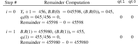
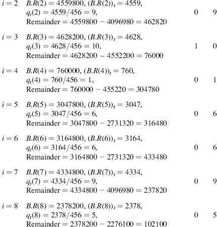
Algorithm 6.10 Nonrestoring Base-B Division Step
rt:=B*r/B**(n-3); yt:=y/B**(n-3);
qt:=rt/yt+1; qt1:=qt/B; qt0:=qt modB;
remainder:=B*r-qt*y;
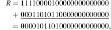
Example 6.7 X and Y are positive 5-digit decimal numbers Compute X/Y as 45598/45522 with an accuracy of p = 7. To ensure that X < Y, a preliminary normalization procedure sets the operands to 045598 and 455220, respectively (n = 6, p = 7 + 1 = 8).
The final correction is expressed as
![]()
and the overall operation can be resumed as
![]()
The decimal system has been used without ambiguity to represent the accuracy in the multiplicative factor 108.
The minimum redundancy of the quotient-digit set allows an easy correction procedure: adding 1 at level i − 1 whenever a quotient-digit q(i) reaches B. The remainder computation is aided by the fact that the remainder is always positive. The tentative quotient-digits may be extracted from look-up tables, or computed by a specific circuit. Instead of computing the remainder as a full k-digit subtraction, a carry-save technique may be applied to store the remainder as the signed sum of two k-digit numbers.