4.1 ADDITION OF NATURAL NUMBERS
4.1.1 Basic Algorithm
Consider the base-B representations of two n-digit numbers:
![]()
The following (pencil and paper) algorithm computes the (n + 1)-digit representation of z = x + y + cin where cin is an initial carry equal to 0 or 1.
Algorithm 4.1 Classic Addition
q(0): =c_in;
for i in 0..n-1 loop
   if x(i)+y(i)+q(i)>B-1 then q(i+1):=1; else q(i+1):=0;
   end if;
   z(i):=(x(i)+y(i)+q(i)) mod B;
end loop;
z(n):=q(n);
As q(i + 1) is a function of q(i) the execution time of Algorithm 4.1 is proportional to n. In order to reduce the execution time of each iteration step, Algorithm 4.1 can be modified. First, define two binary functions of two B-valued variables, namely, the propagate (p) and generate (g) functions:
The next carry qi+1 can be calculated as follows:
if p(x(i), y(i))=1 then q(i+1):=q(i); else q(i+1):=g(x(i),
y(i)); end if;
The corresponding modified algorithm is the following one.
Algorithm 4.2 Carry-Chain Addition
--computation of the generation and propagation conditions:
for i in 0..n-1 loop g(i):=g(x(i),y(i)); p(i):=p(x(i),y(i));
end loop;
--carry computation:
q(0):=c_in;
for i in 0..n-1 loop
  if p(i)=1 then q(i+1):=q(i); else q(i+1):=g(i); end if;
end loop;
-sum computation
for i in 0..n-1 loop z(i):=(x(i)+y(i)+q(i)) mod B; end loop;
z(n):=q(n);
Comments 4.1
- Observe that the first iteration includes 2.n B-ary operations (computation of g(i) and p(i)) that could be executed in parallel. The second iteration is made up of n iteration steps that must be executed sequentially (as q(i + 1) is a function of q(i)) and consists of binary operations only. The last iteration includes n B-ary operations (computation of z(i)) that could be executed in parallel. Algorithm 4.2 thus splits the operations into concurrent B-ary ones (first and third iterations) and sequential binary ones (second iteration). The sequential binary operations are the same whatever the base B. The expected computation time reduction is due to the substitution of the (relatively) complex instruction
if x(i)+y(i)+q(i)>B-1 then q(i+1):=1; else q(i+1):=0;
end if;
by the simpler one
if p(i)=1 then q(i+1):=q(i); else q(i+1):=g(i); end if;
- The preceding instruction sentence is equivalent to the following Boolean equation:
Furthermore, if the preceding relation is used, then the definition of the generate function can be modified:

- Another Boolean equation equivalent to (4.2) is
If the preceding relation is used, then the definition of the propagate function can be modified:

4.1.2 Faster Algorithms
The values of q(1), q(2),…,q(n) could also be calculated in parallel:
Property 4.1
where symbol ∨ stands for the Boolean sum, g(i) = g(x(i), y(i)) and p(i) = p(x(i), y(i)).
Relation (4.4) is deduced from (4.3) by induction. The corresponding algorithm is the following one.
Algorithm 4.3
--computation of the generation and propagation conditions:
for i in 0..n-1 loop g(i):=g(x(i),y(i)); p(i):=p(x(i),y(i));
end loop;
--carry computation:
q(0):=c_in;
for i in 1..n loop
  q(i):=g(i-1) or g(i-2)*p(i-1) or…or g(0)*p(1)*…*
  p(i-1) or q(0)*p(0)*p(1)*…*p(i-1);
end loop;
--sum computation
for i in 0..n-1 loop z(i):=(x(i)+y(i)+q(i)) mod B; end loop;
z(n):=q(n);
The preceding algorithm is made up of three iterations whose operations could be executed in parallel as q(i) just depends on the operands x, y, and c_in but not on the preceding carries. Nevertheless, the execution of
q(i):=g(i-1) or g(i-2)*p(i - 1) or…or g(0)*p(1)*…*p(i-1)
 or q(0)*p(0)*p(1)*…*p(i-1);
implies the computation of a (2.i + 1)-variable switching function—a (2.n + 1)-variable function in the case of q(n). Except for small values of n, specific algorithms must be defined for computing these functions. For that purpose two new concepts are introduced: the dot operation and the generalized generate and propagate functions:
Definitions 4.1
- Given two 2-component binary vectors ai = (ai0, ai1) and ak = (ak0, ak1) the dot operation • defines an application from
 × into :

It can easily be demonstrated that it is a noncommutative associative operation; (0,1) is the neutral element and (0,0) the left 0-element.
- Given the generate and propagation functions g(i) and p(i), for i
 {0, 1,…, n − 1}, the generalized generate and propagate functions g(i:i-k) and p(i:i-k), for i {0, 1,…,n − 1} and k {0, 1,…, i} are defined as follows:
The following property is deduced from (4.4) and from the preceding definitions.
Then Algorithm 4.3 can be modified as follows.
Algorithm 4.4
--computation of the generation and propagation conditions:
for i in 0..n-1 loop g(i):=g(x(i),y(i)); p(i):=p(x(i),y(i));
 end loop;
--computation of the generalized generation and propagation
 conditions:
for i in 1..n loop
  (g(i-1:0), p(i-1:0)):=(g(i-1), p(i-1)) dot (g(i-2),
  p(i-2)) dot … dot (g(0), p(0));
end loop;
--carry computation:
q(0):=c_in;
for i in 1..n loop q(i):=g(i-1:0) or p(i-1:0)*q(0); end loop;
--sum computation:
for i in 0..n-1 loop z(i):=(x(i)+y(i)+q(i)) mod B; end loop;
z(n):=q(n);
The second iteration of Algorithm 4.4, that is, the computation of all pairs (g(i − 1, 0), p(i − 1, 0)), can be performed in several ways. It is a particular case of a more general problem: Given a set of input data a(0), a(1),…, a(n − 1) and an associative operator • (dot), compute

The simplest (naïve) algorithm is
b(0):=a(0); for i in 1..n−1 loop b(i):=a(i) dot b(i − 1); end loop;
whose execution time is proportional to n. Nevertheless, better algorithms have been proposed, among others ([BRE1982], [LAD1980], [KOG1973], [HAN1987], [SUG1990]). Two of them are described below; they are based on the definition of a procedure dot_procedure computing Equations (4.7); its input and output parameters are a natural number n (the number of input data), and two n-component vectors (the input data and the output result):
procedure dot_procedure (n:in natural;
a:in data_vector(0..n-1); b:out data_vector(0..n-1));
Assume that n is a power of 2 (0's should be added if necessary). A first algorithm consists of:
computing

colling dot_procedure with parameters n/2, c, and d, so that

computing the missing components of b;
![]()
The computation scheme (or precedence graph, Chapter 10) is shown in Figure 4.1 (with n = 16). The corresponding recursive algorithm is the following.
Algorithm 4.5 Dot Procedure (1)
procedure dot_procedure (n:in natural; a:in data_vector(0..
n-1); b: out data_vector(0..n-1)) is
  c,d: data_vector(0..(n/2)-1);
begin
  if n=2 then b(0):=a(0); b(1):=a(1) dot a(0);
  else
  for i in 0..(n/2)-1 loop c(i):=a((2*i)+1) dot a(2*i);
  end loop;
  dot_procedure (n/2, c, d);
  b(0):=a(0);
  for i in 1..(n/2)-1 loop b(2*i):=a(2*i) dot d(i-1);
  b((2*i)+1):=d(i); end loop;
  end if;
end dot_procedure;

Figure 4.1 A 16-input dot procedure (first algorithm).
Both for loops are made up of dot operations that can be executed in parallel. The total execution time T(n) is equal to Tdot + T(n/2) + Tdot, with T(2) = Tdot, so that
The second algorithm consists of:
calling dot_procedure with parameters n/2, a(0 ..(n/2) − 1), and b(0 . .(n/2) − 1);
calling dot_procedure with parameters n/2, a((n/2) . . n − 1), and c, so that

computing the missing components of b,

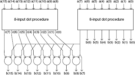
Figure 4.2 A 16-input dot procedure (second algorithm).
The computation scheme is shown in Figure 4.2 (with n = 16), and the corresponding recursive algorithm is the following.
Algorithm 4.6 Dot Procedure (2)
procedure dot_procedure (n:in natural; a:in data_vector(0..
n-1);b:out data_vector(0..n-1)) is
  c: data_vector(0..(n/2)-1);
begin
  if n=2 then b(0):=a(0); b(1):=a(1) dot a(0);
  else
   dot_procedure (n/2, a(0..(n/2)-1), b(0..(n/2)-1);
   dot_procedure (n/2, a((n/2)-1..n-1), c);
   for i in 0..n/2-1 loop b(i+(n/2)):=c(i) dot b((n/2)-1);
   end loop;
  end if;
end dot_procedure;
Both procedure calls can be executed in parallel, and the for loop is made up of dot operations that can also be executed in parallel. The total execution time T(n) is equal to T(n/2) + Tdot, with T(2) = Tdot, so that
The following algorithm is deduced from Algorithm 4.4 and the definition of dot_procedure.
Algorithm 4.7 Parallel-Prefix Addition
a, b: data_vector(0..n-1, 0..1);
begin
  --computation of the generation and propagation conditions:
  for i in 0..n-1 loop a(i,0):=g(x(i),y(i)); a(i,1):=p(x(i),
   y(i))); end loop;
  --computation of the generalized generation and propagation
  --conditions:
  dot_procedure(n, a, b);
  --carry computation:
  q(0):=c_in;
  for i in 1..n loop q(i):=b(i,0) or b(i,1)*q(0); end loop;
  --sum computation
  for i in 0..n-1 loop z(i):=(x(i)+y(i)+q(i)) mod B; end loop;
  z(n):=q(n);
The preceding algorithm is made up of three iterations, whose operations can be executed in parallel, and a call to dot_procedure. The procedure execution time depends on the number of digits n; according to (4.8) or (4.9) it is proportional to log(n). The execution time of the iterations is independent of n. Thus for great values of n, the execution time of Algorithm 4.7 is practically proportional to log(n).
A logarithmic execution time can be obtained with a different algorithm using two new procedures. The first one,
procedure carry_lookahead_procedure (n: in natural; a: in data_
vector(0..n-1, 0..1); c_in: in bit; q: out bit_vector(1..n));
computes the n carries q(1), q(2), …, q(n), in function of the n generation and propagation conditions g(t) = a(t,0) and p(t) = a(t,1), and of c_in, that is,
![]()
The second one,
procedure carry procedure (n:in natural; b:in data_vector(0..
n-1, 0..1); c_in: in bit; q: out bit_vector(1..n));
computes the n carries q(1), q(2),…, q(n), in function of the n generalized generation and propagation conditions g(t:0) = b(t,0) and p(t:0) = b(t,1), and of c_in, that is,
Assume that n can be factorized under the form n = k.s. The algorithm consists of:
calling k times the dot_procedure with parameters s, a(j.s .. j.s + s − 1) and c(j,0. .s − 1), where j ![]() {0, 1,…, k − 1}, so that
{0, 1,…, k − 1}, so that

calling carry_lookahead_procedure with parameters k, c(0 . . k − 1, s − 1), c_in and d, so that
![]()
calling k times the carry_procedure with parameters s − 1, c(j, 0.. s − 2), d(j), and e(j,0 . . s − 2), where j ![]() {0, 1,…, k − 1}, so that
{0, 1,…, k − 1}, so that
![]()
The computation scheme is shown in Figure 4.3 (with k = s = 4), and the corresponding recursive algorithm is the following:
Algorithm 4.8
procedure carry_lookahead_procedure
(n:in natural; a:in data_vector(0..n-1, 0..1); c_in: in bit;
q:out bit_vector(1..n)) is
  c: data_vector(0..k-1, 0..s-1, 0..1); d: bit_vector(0..
  k-1);
begin
  for j in 0..k-1 loop dot_procedure(s, a(j*s..j*s+s-1), c(j,
  0..s-1)); end loop;
  carry_lookahead_procedure (k, c(0..k-1, s-1), c_in, d);
  for j in 0..k-1 loop
    carry_procedure(s-1, c(j, 0..s-2), d(j), e(j, 0..s-2));
  end loop;
  for j in 1..k-1 loop q(j*s):=d(j); end loop;
  for j in 0..k-1 loop
    for i in 0..s-2 loop q(j*s+i+1):=e(j, i); end loop;
  end loop;
end carry_lookahead_procedure;

Figure 4.3 A 16-input carry_lookahead_procedure.
The procedure carry_procedure computes (4.10):
procedure carry_procedure
(n:in natural; b:in data_vector(0..n − 1, 0..1) c_in: in bit;
q:out bit_vector(1..n))
is begin
  for t in 1..n loop q(t)=b(t − 1,0) v c_in.b(t − 1,1); end loop;
end carry_procedure;
Let T(n) be the execution time of carry_lookahead_procedure, T1(n) the execution time of dot_procedure, and T2 the execution time of any one of the equations (4.10). The k calls to dot_procedure can be executed in parallel, and the same occurs with the k calls to carry_procedure. Furthermore, within carry_procedure the equations (4.10) can be calculated in parallel. Thus
![]()
Assume now that n = s1. s2. … . sm. The algorithm obtained by recursively calling the carry_lookahead_procedure has a computation time that can be calculated as follows:

so that
In particular, if n = sm then
The complete addition algorithm is the following.
Algorithm 4.9 Carry-Lookahead Addition
a: data_vector(0..n-1, 0..1);
begin
  --computation of the generation and propagation conditions:
  for i in 0..n-1 loop a(i,0):=g(x(i),y(i)); a(i,1):=p(x(i),
   y(i))); end loop;
  --carry computation
  carry_lookahead_procedure(n, a, c_in, q);
  q(0):=c_in;
  --sum computation
  for i in 0..n-1 loop z(i):=(x(i)+y(i)+q(i)) mod B; end loop;
  z(n):=q(n);
4.1.3 Long-Operand Addition
In the case of long-operand additions it may be necessary to break down the n-digit operands into s-digit slices. A typical example is the implementation of n-bit arithmetic operations within an m-bit microprocessor, with m < n. Taking into account that an n-digit base-B number can also be considered as being an (n/s)-digit base-Bs number (Comment 3.1) a modified version of the basic algorithm 4.1 can be used. The iteration body of Algorithm 4.1 must be substituted by a procedure natural_addition, which computes the sum of two s-digit numbers:
procedure natural_addition (s: in natural; carry: in bit; x, y:
in digit_vector(0..s-1); next_carry: out bit; z: out digit_
vector(0..s-1);
Any one of the previously proposed algorithms (4.1, 4.2, 4.7, or 4.9) can be used for defining the natural_addition procedure. Then the following algorithm computes x + y + cin.
Algorithm 4.10 Long-Operand Addition
q:=c_in;
for i in 0..n/s-1 loop
  natural_addition(s, q, x(i*s..(i*s)+s-1), y(i*s..(i*s)+s-1),
   q, z(i*s..(i*s)+s-1));
end loop;
z(n):=q;
Depending on the selection of the natural_addition procedure, the corresponding execution time is proportional to either (n/s).s = n or (n/s).log s.
Observe that modified versions of the other algorithms would not give shorter execution times: all of them include n sentences
z(i):=(x(i)+y(i)+q(i)) mod B;
equivalent, in base Bs, to n/s sentences
natural_addition(s, q(i), x(i*s..(i*s)+s-1), y(i*s..(i*s)+
s-1), not_used, z(i*s..(i*s)+s-1));
As the n/s preceding sentences must be executed sequentially (long-operand constraint), the execution time would still be proportional to either (n/s).s = n or (n/s).log(s).
4.1.4 Multioperand Addition
Another important operation is the multioperand addition, that is, the computation of z = x(0) + x(1) + … + x(m−1), where every x(i) is a natural number. Assume that the overall sum z does not exceed n digits and that all operands are expressed with n digits. The following algorithm computes z.
Algorithm 4.11 Basic Multioperand Addition
accumulator:=0;
for j in 0..m-1 loop
  natural_addition(n, 0, accumulator, x(j), not_used,
  accumulator);
end loop;
z:=accumulator;
Its execution time is proportional to m.n or m.log n depending on the selected natural_addition procedure.
An interesting concept for executing multioperand additions is the stored-carry form encoding of the result of a 3-operand addition. Assume that a procedure
procedure three-to-two(w, x, y: in natural; u, v: out natural);
has been defined; it computes u and v such that
![]()
Then the following algorithm computes the sum z = x(0) + x(1) + … + x(m−1) of m natural numbers.
Algorithm 4.12
three-to-two(x(0), x(1), x(2), u(0), v(0));
for j in 3..m-1 loop
  three-to-two (x(j), u(j-3), v(j-3), u(j-2), v(j-2));
end loop;
natural_addition(n, 0, u(m-3), v(m-3), not_used, z);
The three-to-two procedure consists in expressing the sum z of three natural numbers (w, x, y) under the form of a pair (u, v) of two natural numbers in such a way that z = u + v. Assume now that w, x, and y are n-digit numbers, and q_in is a 1-digit number. The following algorithm computes two n-digit numbers u and v, and a 1-digit number q_out, such that
Algorithm 4.13 Stored-Carry Encoding
procedure stored-carry_encoding(w, x, y: in digit_vector(0..
n-1); q _in: in digit; u, v: out digit_vector(0..n-1); q _out:
out digit) is
begin
  q(0):=q _in;
  for i in 0..n-1 loop
    q(i+1):=(w(i)+x(i)+y(i))/B;
    u(i):=(w(i)+x(i)+y(i)) mod B;
  end loop;
  v:=q(0..n-1); q_out:=q(n);
end stored-carry_encoding;
Algorithm 4.13 is similar to the basic addition algorithm 4.1: two digits are computed at each step, and the first one, q(i + 1), can be considered as a B-ary carry (instead of a binary one when B > 2). Nevertheless, q(i + 1) does not depend on q(i) so that the n iteration steps can be executed in parallel. In other words, at each step the carry q(i + 1) is stored instead of being transferred to the next iteration step. For that reason the pair (u, v) is said to be the stored-carry form of z.
The following multioperand algorithm, where x(j, i) stands for x(j)(i) is deduced from Algorithms 4.12 and 4.13 (assuming that z is an n-digit number and that all operands are expressed with n digits).
Algorithm 4.14 Carry-Save Addition
stored-carry_encoding(x(0, 0..n-1), x(1, 0..n-1), x(2,
0..n-1), 0, u(0, 0..n-1), v(0, 0..n-1), not_used);
for j in 3..m-1 loop
  stored-carry_encoding (x(j,0..n-1), u(j-3, 0..n-1),
  v(j − 3, 0..n-1), 0, u(j-2, 0..n-1),
  v(j-2, 0..n-1), not_used);
end loop;
z(0):=u(m-3, 0);
natural_addition(n-1, 0, u(m-3, 1..n-1), v(m-3, 1..n-1),
 not_used, z(1..n-1));
The carry-save addition algorithm is made up of m − 2 calls to stored-carry_encoding and a call to an (n − 1)-digit addition procedure, so that the execution time is roughly proportional to m + n or m + log(n), instead of m.n or m.log(n).
Comments 4.2
- Instead of the three-to-two procedure, more general p-to-k procedures could be defined, as well as multioperand addition algorithms in which p − k new operands are added at each step. The generalized version of Algorithm 4.12 would include m ≅ (n − k)/(p − k) steps to reach k operands. Each step could be decomposed in a similar way as in the case of Algorithm 4.13. For instance, with p = 7 and k = 3, each step of the generalized algorithm 4.12 should compute the sum of seven numbers w(0), w(1),…, w(6), and encode the result as a three-component vector; the generalized version of Algorithm 4.13 should compute
q(i+2):=(w(0, i)+w(1, i)+···+w(6, i))/(B**2);
r(i+1):=(w(0, i)+w(1, i)+···+w(6, i)-q(i+2)*(B**2))/B;
u(i):=(w(0, i)+w(1, i)+···+w(6, i)) mod B;
at each iteration step (observe that if B ≥ 2, then 7.(B − 1) < B2). This idea, mainly applicable to the case of hardware implementations, will be developed in Chapter 11.
- Another idea mainly applicable to hardware implementations is the substitution of the iterations (as in Algorithms 4.11, 4.12, and 4.14) by tree structures. It will also be developed in Chapter 11.
4.1.5 Long-Multioperand Addition
A long-multioperand addition can be executed by combining Algorithms 4.10 and 4.11.
Algorithm 4.15
accumulator:=0;
for j in 0..m-1 loop
  q:=0;
  for i in 0..n/s-1 loop
    natural_addition(s, q, accumulator(i*s..(i*s)+s-1),
    x(j,i*s..(i*s)+s-1), q, accumulator(i*s..(i*s)+s-1));
  end loop;
end loop;
z:=accumulator;
Its execution time is proportional to either m.(n/s).s = m.n or m.(n/s).log(s).
The stored-carry encoding could be used too. The reduction of m n-digit operands to 2 n-digit operands can be performed by breaking down each n-digit operand into n/s s-digit ones and calling the stored-carry_encoding procedure (m − 2).(n/s) times. Then the so-obtained operands are added.
Algorithm 4.16 Carry-Save Long-Multioperand Addition
--m-to-2 reduction:
q:=0;
for i in 0..n/s-1 loop
  stored-carry_encoding (x(0, i*s..(i*s)+s-1),
  x(1, i*s..(i*s)+s-1), x(2, i*s..(i*s)+s-1),
  q, u(i*s..(i*s)+s-1), v(i*s..(i*s)+s-1), q);
end loop;
for j in 3..m-1 loop
  q:=0;
  for i in 0..n/s-1 loop
    stored-carry_encoding (x(j, i*s..(i*s)+s-1), u(i*s..(i*s)
    +s-1), v(i*s..(i*s)+s-1),q, u(i*s..(i*s)+s-1),
    v(i*s..(i*s)+s-1), q);
  end loop;
end loop;
--2-operand addition:
q:=0;
for i in 0..n/s-1 loop
  natural_addition(s, q, u(i*s..(i*s)+s-1), v(i*s..(i*s)+
  s-1), q, z(i*s..(i*s)+s-1));
end loop;
The m-to-2 reduction is performed in (m − 2).(n/s) steps, and the 2-operand addition execution time is proportional to either (n/s).s = n or (n/s).log s. The total execution time is roughly proportional to either (n/s).(m + s) or (n/s).(m + log s) instead of (n/s).m.s or (n/s).m.log s.