14.6 SQUARE ROOTERS

This section presents implementations of binary square rooters based on restoring shift-and-subtract Algorithm 7.12, nonrestoring shift-and-subtract Algorithm 7.13, and the Newton–Raphson method of Section 7.4.4.

14.6.1 Restoring Shift-and-Subtract Square Rooter (Naturals)

The circuits presented in Figures 14.20 and 14.21, implementing Algorithm 7.12, are somewhat similar to the restoring divider presented in Chapter 13. Binary 2's complement notation is assumed. The restoring process is achieved by a multiplexer selecting the previous remainder in case of a negative result from the subtraction step. The key difference rests on the expression P(i) to be subtracted from the successive remainder R(i − 1). The final result Q(−1) is built up by concatenation of the complemented sign bits, from q(n − 1) to q(0). The function P(i) is computed as (formula (7.82) of Chapter 7)

To achieve this function (14.38), pseudo-operators are displayed in Figure 14.20 as shifters: they stand for the rules to be respected to connect Q(n − i) to the subtractor input P(i); input P(i) is made up of Q(n − 1), followed, from left to right, by the string ‘01’ then by a string of 2.(n − i) zeros.

At step 1, registers are initialized as

Figure 14.20 Restoring 2n-bit square rooter, combinational implementation.

After n steps the integer square root of X and the remainder R are stored as

The cost and computation time of a combinational 2n-bit square rooter (n-bit square root), as shown in Figure 14.20, are given by

where T_mux2 is assumed greater than the inverter delay.

The sequential implementation presented in Figure 14.21 needs a nontrivial indexed shifter device to connect Q(n − i − 1) to the subtractor input, through register P(i + 1). Synchronized registers ensure one digit per step. The cost and computation time of a sequential 2n-bit square rooter (n-bit square root), as shown in Figure 14.21, are given by

Figure 14.21 Restoring 2n-bit square rooter, sequential implementation.

14.6.2 Nonrestoring Shift-and-Subtract Square Rooter (Naturals)

The circuits presented in Figures 14.22 and 14.23, implementing Algorithm 7.13, are somewhat similar to the nonrestoring divider presented in Chapter 13. Binary 2's complement notation is assumed. The nonrestoring feature brings on two main differences with respect to the circuits of Figures 14.20 and 14.21. One first observes that the arithmetic cell is now an adder/subtractor whose operation (Add/Subtract) is controlled by the sign of the preceding partial remainder. The other key difference rests on the expression P(i) to be added/subtracted from the successive remainder R(i − 1). The final result Q(−1) is still built up by concatenation of the complemented sign bits, from q(n − 1) to q(0). Function P(i) is now computed as (formulas (7.90) and (7.91) of Chapter 7)

or

Formulas (14.43) and (14.44) may be merged as

This allows the use of a unique set of connecting rules materialized by the pseudo-operators (shifters) in Figure 14.22 or the indexed shifters in Figure 14.23.

At step 1, registers are initialized as

As X is positive, the first arithmetic operation is a subtraction: R(0) − P(1). After n steps the integer square root of X and the remainder R are stored as

If R(n) is negative, the final remainder needs to be adjusted to the last positive partial remainder. The cost and computation time of a combinational 2n-bit square rooter (n-bit square root), as shown in Figure 14.22, are given by

The sequential implementation presented in Figure 14.23 needs an indexed shifter device to connect Q(n − i − 1) to the subtractor input, through register P(i + 1).

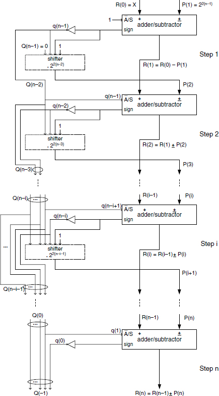
Figure 14.22 Nonrestoring 2n-bit square rooter, combinational implementation.

Figure 14.23 Nonrestoring 2n-bit square rooter, sequential implementation.

Synchronized registers ensure one digit per step. The cost and computation time of a sequential 2n-bit square rooter (n-bit square root), as shown in Figure 14.23, are given by

14.6.3 Newton–Raphson Square Rooter (Naturals)

The iteration equation (7.96)

converges toward the inverse square root 1/X^1/2. A dedicated implementation is depicted in Figure 14.24. The iteration step involves one squaring unit, two multipliers, and one dedicated (3's complement) subtractor. A pseudo-operator (shifter) stands for a right-shift operation, readily achieved by an appropriate loop- connection to the multiplexer represented in the general structure of Figure 14.24. The operators are designed according to the required precision p. A look-table (LUT), addressed by the truncated argument X_t, provides a first t-bit evaluation of 1/X^1/2; its dimension is (roughly) t.2^t bits.

The outputs of the operators are rounded up at the required precision p; several bits may be added to cope with rounding and error propagation. The argument length is assumed not greater than 2p. Although the argument is a natural number, the intermediate results, as well as the final one, are not. Floating-point notation is recommended to optimize the overall precision. Example 14.2 illustrates this point.

Figure 14.24 Newton–Raphson iteration circuit: 2p-bit square rooter.

Example 14.2 Let

Assume that the LUT value x(0) of 1/X^1/2 is 11.2⁻⁵, 2-bit approximation corresponding to the inverse of root of the truncated 2-bit value X_t = 01100000 (rounded up). The following table shows the first two steps of computation with rounding to 16 bits.

After step 2 (i = 1), the approximation of X^1/2 is

showing 10-bit accuracy.

The cost and computation time of the Newton–Raphson square rooter (p-bit square root), as shown in Figure 14.24, are given by

where k = log₂ (p/t).

Comment 14.1 An important question about algorithms using look-up tables, and convergence algorithms in particular, is the evaluation of the exact (i.e., minimum) amount of bits necessary for any prescaling or intermediate calculations to ensure a correct result within the desired precision. Theoretically, the Newton–Raphson algorithms provide a quadratic convergence rate, doubling the number of exact bits at each step. In practice, the accuracy of the look-up tables together with the rounding errors could slow down that rate, unless additional bits are provided to represent LUT data and intermediate results. Actually, the accurate calculus of rounding errors is not a straightforward matter. This mathematical problem has been treated extensively in the literature ([COR1999], [DAS1995], [TAN1991]). Using extra-bits is a safe and easy way to ensure correctness; nevertheless, a careful error computation can lead to significant savings.