7.4 SQUARE ROOTING

Square rooting deserves special attention because of its frequent use in a number of applications ([ERC1994], [OBE1999]). Although square rooting can be viewed as a particular case of the exponential operation, the similarity with division is a more important consideration for the choice of algorithms. Several techniques in base-B and in binary systems are reviewed in this section.

7.4.1 Digit Recurrence Algorithm—Base-B Integers

Let

be the 2n-digit base-B radicand.

The square root Q and the remainder R are denoted

and

respectively.

The remainder

TABLE 7.8 cos 30°, sind 30°

complies with the condition

ensuring that

The classical pencil and paper method, described in what follows, assumes that all roots of 2-digit numbers are available ((B² − 1) × (B − 1) look-up table). Allowing the first digit of X to be zero, the radicand can always be sliced into n 2-digit groups. Algorithm 7.11 computes the square root of the 2n-digit integer X. The symbol * stands for integer multiplication, while ** and / stand for integer exponentiation and division respectively. One defines the function P(i, k) as

Algorithm 7.11 Integer Square Rooting in Base B

R(0):=X; Q(n−1):=0;
q(n−1):=SQR (R(0)/B**(2*n-2));
Q(n-2):=q(n−1);
R(1):=R(0)-(q(n−1)**2)*(B**(2*n-2));

for i in 2..n loop
  if P(i, B-1)<=R(i-1) then R(i):=R(i-1)-P(i, B-1);
  q(n-i):=B-1;
  Q(n-i-1):=B*Q(n-i)+q(n-i);
  elsif P(i, B-2)<=R(i) then R(i):=R(i-1)-P(i, B-2);
  q(n-i):=B-2;
  Q(n-i-1):=B*Q(n-i)+q(n-i);
  elsif
  …
  elsif P(i, 1) <=R(i) then R(i):=R(i-1)-P(i, 1); q(n-i):=1;
  Q(n-i-1):=B*Q(n-i)+q(n-i);
  else R(i):=R(i-1); q(n-i):=0; Q(n-i-1):=B*Q(n-i)+q(n-i);
  end if;
end loop;

Example 7.12 Compute the square root of X = (591865472)₁₀

Slicing (n = 5) gives X = R(0) = 05 '91 '86 '54 '72

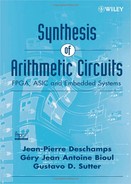
Step 1

Step 2

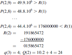
Step 3

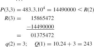
Step 4

Step 5

Comments 7.6 The process can be carried on further, up to the desired quantity of digits after the decimal point.

The function P(i, k) (7.75) of Algorithm 7.11 is used to compute the greatest value of k verifying P(i, k) ≤ R (i − 1).

Actually, k can be defined algebraically by the formula

the integer part of the solution to such that

where

Obviously formula (7.76), using the square root, is useless for algorithmic implementation. Other methods must therefore be derived to get k verifying (7.78).

Techniques for square rooting in base B > 2 are quite similar to those for base-B division. The recurrence formula for the remainder is given by

with

for 2n-digit integers.

7.4.2 Restoring Binary Shift-and-Subtract Square Rooting Algorithm

In base 2, the computation of the function P(i, k) is obviously more straightforward, since just 0 or 1 have to be considered for k. Moreover, since P(i, 0) = 0, just P(i, 1), hereafter denoted P(i), is computed,

Defining

Algorithm 7.11 can be simplified as follows.

Algorithm 7.12 Integer Binary Square Rooting; Restoring

R(0):=X; Q(n−1):=0; q(n):=0; P(1):=2**(2*(n−1));
for i in 1..n, loop
  if R(i−1)-P(i)>=0
  then R(i):=R(i−1)-P(i); q(n-i):=1;
  Q(n-i−1):=2*Q(n-i)+q(n-i);
  else R(i):=R(i−1); q(n-i):=0; Q(n-i−1):=2*Q(n-i)+
  q(n-i);
end if;
end loop;

Example 7.13 Compute the square root of

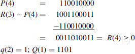
Step 1

Step 2

Step 3

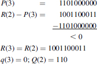
Step 4

Step 5

Step 6

Comments 7.7

1. Generality is not lost assuming 2n digits for the radicand X; a first digit zero can always be assumed.
2. Step 1 of Algorithm 7.12 actually computes q(n-1) as the integer square root of the leftmost two bits of the radicand X. If X is not headed by “00”, q(n−1) will always be one.

7.4.3 Nonrestoring Binary Add-and-Subtract Square Rooting Algorithm

As well as in the classical binary division algorithm, restoring the remainder, whenever negative, is not necessary since the following operation can cope with a negative remainder and perform in a single operation the restoring process together with the next step operation.

Considering a current step i, notice that when

the nonrestoring algorithm proceeds like the restoring one.

Whenever

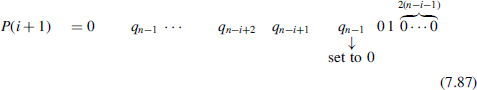
the restoring process would add back P(i) to the partial result (7.84), set q(n − i) to zero, then subtract P(i + 1) from restored R(i − 1). These operations can be substituted by adding, to the partial result (7.84), the following expression

at the next step i + 1.

Since, from step i (7.84), q(n − i) = q_n−i = 0, one can write:

and

then

Assuming

(7.88) can be written

The nonrestoring binary square rooting method is described in Algorithm 7.13, where P(i) and Pstar(i) are defined as follows

Algorithm 7.13 Integer Binary Square Rooting; Nonrestoring

  R(0):=X; Q(n−1):=0; q(n):=0; P(1):=2**(2*(n−1));
  R(1):=R(0)-P(1);
  if R(1)>=0
  then q(n−1):=1; Q(n-2):=1;
  else q(n−1):=0; Q(n-2):=0;
  end if;
  for i in 2..n loop
     if R(i-1)>=0
     then R(i):=R(i-1)-P(i);
     else R(i):=R(i-1)+Pstar(i);
     end if;
     if R(i)>=0
     then q(n-i):=1; Q(n-i-1):=2*Q(n-i)+q(n-i);
     else q(n-i):=0; Q(n-i-1):=2*Q(n-i)+q(n-i);
     end if;
end loop;

As well as for nonrestoring division algorithms, a final correction may be necessary. Whenever the final remainder is negative, it needs to be adjusted to the previous positive one.

Example 7.14 Note: 2's complement notation is used; the sign bit is in boldface type

Compute the square root of

Step 1

Step 2

Step 3

Step 4

Step 5

Step 6

Step 7

the exact square root.

Comments 7.8 The square rooting methods developed in the preceding sections are classic and easy to implement. The main component involved in the step complexity is the signed sum. One digit is obtained at each step (digit recurrence), so, for a desired precision p, p n-digit adding stages are involved, combinationally or sequentially implemented. To speed-up the process, fast adders may be used. SRT type algorithms have been developed for square rooting, using the feature of carry-save redundant adders ([ERC2004]). On the other hand, convergence algorithms have been developed, such as Newton–Raphson, reviewed in the following section.

7.4.4 Convergence Method—Newton–Raphson

The priming function for square root computation could be

which has a root at x=X^1/2.

To solve f(x)=0, the same equation used for inverse computation can be used:

or

Formula (7.94) involves a division and an addition at each step, which makes Newton–Raphson's method apparently less attractive in this case. Nevertheless, computing the inverse square root 1/X^1/2, then multiplying by the radicand X, leads to a more effective solution.

The priming function is now

with root x=1/X^1/2, and the equation of convergence is given by

which involves three multiplications, one subtraction (3's complement), and one division by 2 (shift in base 2). A final multiplication is needed: the inverse square root by the radicand.