WPF is essentially a two-dimensional technology. The panel-based layout system knows how to arrange 2D elements onto a 2D screen. Likewise, the flow document system knows how to flow text onto a two-dimensional page. So how does 3D content fit into this world?

The Viewport3D element bridges the gap between 2D and 3D. As far as the WPF layout system is concerned, Viewport3D is just a rectangular element. It is similar in nature to the MediaElement type: both are rectangular elements that can display moving images. Whereas MediaElement displays a recorded video stream, a Viewport3D works more like a live video feed from a camera—a virtual camera in a 3D model.

Viewport3D fits into the WPF layout model like any other element. You can give it an explicit width and height, or you can let it pick up its height from a containing panel such as a Grid. You can host it inside a panel or a content control just like any other element. And, of course, all the normal layout properties, such as Margin and HorizontalLayout, are available.

Viewport3D requires us to supply three things: a camera description, one or more light sources, and a 3D model. Without a model, there is nothing to display. Without a light source, there is no way to see the model. And, the Viewport3D needs a camera description so that it knows the point of view from which it should render the scene.

You must set the Viewport3D’s Camera property to one of the three available camera types: PerspectiveCamera, OrthographicCamera, or MatrixCamera. The type of camera determines how the 3D model will be turned into a 2D image on-screen.

The PerspectiveCamera is often the most natural choice. With this camera, the farther away objects are, the smaller they appear. Because that’s how things look in real life, this produces a reasonably natural-looking image.

The OrthographicCamera uses a more simplistic approach. A 3D object of a particular size will always be rendered at exactly the same size, regardless of how far away it is. This tends to produce rather unnatural-looking images, but it can occasionally be useful—sometimes consistency is more important than a natural appearance. If you are rendering 3D models representing the design of something physical, such as a planned piece of woodwork or the layout of a room, you might want objects of the same size in the model to appear the same size on-screen. Likewise, if you are producing a 3D graph, consistency of size might be more important than realism. An OrthographicCamera can guarantee this, whereas a PerspectiveCamera can, by design, show equal-size objects as different sizes on-screen. Figure 17-1 shows an example—on the left is a series of identical columns rendered with a PerspectiveCamera, and on the right is the same model as shown by an OrthographicCamera.

Figure 17-1. PerspectiveCamera and OrthographicCamera

If you are using either the PerspectiveCamera or the OrthographicCamera, you need to provide information about the camera’s position and orientation. You set its location relative to the coordinate space of the Viewport3D’s model with the Position property. The LookDirection property indicates which direction the camera is pointing. This isn’t quite enough to establish the camera’s orientation—a camera in a particular location pointed in a particular direction can still be rotated around the axis in which it is pointing. For example, when taking a photograph with a real camera, you can rotate it to choose between a portrait or landscape shot. So, you must also specify an UpDirection.

This pins down the location and orientation of the camera, but you still need to indicate how wide a shot you require. (In real camera terms, this is equivalent to adjusting the focal length of a zoom lens.) With the PerspectiveCamera, you do this with the FieldOfView property, specifying an angle in degrees. Narrowing the angle has the effect of zooming in, and increasing the angle zooms out.

Example 17-1 shows a PerspectiveCamera. This is positioned and oriented such that the model’s x- and y-axes will appear horizontal and vertical in the Viewport3D, respectively. The camera is looking directly at the origin, and it is positioned on the z-axis itself, four units away from the origin in the positive z direction. The position we’ve chosen for this camera means that lower values of z are farther away from the camera.

<PerspectiveCamera Position="0,0,4" LookDirection="0,0,−1"
                      UpDirection="0,1,0" FieldOfView="45" />

To demonstrate the impact of the various camera settings, we’ll look at how making small changes to each property affects what the camera sees. The model in all cases will be the same. It will consist of five cylinders, similar to those shown in Figure 17-1, but with a couple of the cylinders colored black to make it easier to see which way around things are—with a 3D view it is possible to look at a scene from any angle, so it’s useful to have something to help keep your bearings. Figure 17-3 shows a plan view of the model viewed from above.

The cylinders are positioned in a line near the center. Figure 17-3 also shows a symbol that appears three times toward the bottom—a circle with a cross through it. These indicate camera locations, and the arrow indicates the direction in which the camera is pointing (i.e., the LookDirection). The middle one corresponds to the camera in Example 17-1, and the ones on either side correspond to similar cameras, but with the Position property modified to −1,0,4 and 1,0,4. This is equivalent to moving the camera one unit to the left or one unit to the right. Figure 17-2 shows the three camera positions. The leftmost image shows the leftmost camera position, which results in the leftmost column appearing in the center of the frame, because that column appears directly in front of the camera. Likewise, the rightmost image has the rightmost column dead center, as it is directly in front of the camera. The middle image may look surprising, as it appears slightly lopsided. However, this is just the effect of perspective. The central column is in the center of the frame, and the columns on the right appear nearer to the center than those on the left simply because they are farther away.

Figure 17-2. Position: −1,0,4; 0,0,4; and 1,0,4

Figure 17-3. Model and camera positions

By changing just the Position, we adjust the camera location without changing the direction in which it is pointing. In cinematic terminology, this is equivalent to a tracking shot, in which the camera is typically on rails so that it can move around. With a real camera, an alternative to moving around is to use a panning shot, where the camera remains stationary, but the direction in which it points changes. We can achieve this effect in WPF by changing the camera’s LookDirection. In Figure 17-4, the Position is the same for all three shots—it is back at 0,0,4. Instead, the LookDirection has been adjusted to point the camera at the leftmost column, the central column, and the rightmost column. The difference between this and Figure 17-2 is subtle, but clear—the effect of perspective is different. In Figure 17-2, the columns in the lefthand shot are bunched together fairly closely, and the spacing increases as the camera moves to the right. This effect is sometimes called parallax, and it occurs with any tracking shot. But in Figure 17-4 this effect does not occur, because the camera has not moved; again, with a real camera, parallax effects do not occur with panning shots.

Figure 17-4. LookDirection: −0.33,0,−1; 0,0,−1; and 0.33,0,−1

The third property in Example 17-1 is UpDirection. On a real camera, this would correspond to tilting the camera while keeping it pointed in the same direction. Figure 17-5 shows the effect of changing this property.

Figure 17-5. UpDirection: −0.5,1,0; 0,1,0; and 0.5,1,0

The final property in Example 17-1 is FieldOfView. This has the same effect as changing the focal length of the lens on a real camera, either by adjusting the zoom or by changing lenses. Figure 17-6 shows three shots where all the parameters are the same as in Example 17-1, except for the FieldOfView.

Figure 17-6. FieldOfView: 65; 45; and 25

A zoom facility may seem redundant in a virtual 3D model, because it’s very easy to move the camera around. However, moving a camera close to an item has a different effect than zooming in. The closer a camera gets to its subject, the more distortion is caused by perspective effects. Fitting a very wide angle lens, such as a so-called “fisheye” lens, to a real camera will take this to extremes, producing strangely distorted-looking images. Moving a PerspectiveCamera farther away from a subject and then zooming back in by narrowing the FieldOfView will reduce the effects of perspective. Figure 17-7 shows three shots where the Position has been adjusted to move the camera away from or toward the scene, but the FieldOfView has been adjusted so that the whole model remains in shot and at about the same size, in all three cases. As you can see, the farther away from the model the camera is, the less effect perspective has.

Figure 17-7. Position/FieldOfView: 0,0,2/108; 0,0,4/45; and 0,0,8/20

Although most of the camera settings described apply to the OrthographicCamera, the OrthographicCamera doesn’t adjust objects’ sizes for perspective, so a field-of-view angle would make no sense for this camera. Instead, it has a Width property, which serves a similar purpose—it determines how wide a view the camera takes—but rather than taking an angle, it takes a size, measured in the coordinate space of the 3D model. Figure 17-8 shows the same scene as the previous examples, with the same Position, LookDirection, and UpDirection, but shown by an OrthographicCamera with various Width settings.

Figure 17-8. Width: “5”; “4”; and “3”

The other camera type is MatrixCamera. This lets you define the camera with a pair of matrix transformations. The first, the ViewMatrix, determines the position and orientation of the camera (i.e., it has the same effect as the Position, LookDirection, and UpDirection). The second, the ProjectionMatrix, determines how the image is projected onto the 2D output, including any adjustments for perspective.^[114] You can re-create the effect of either a PerspectiveCamera or an OrthographicCamera.

The MatrixCamera is harder to set up than the other two camera types—4×4 matrix values are rather cryptic compared to position and direction properties. The main reason the MatrixCameraexists is that this matrix representation is fairly common in 3D graphics packages. If you already have code that knows how to set up a camera this way, you can plug the matrices it generates directly into a MatrixCamera.

A camera is not much use without something to look at. So, we must add a model to the Viewport3D.

We describe three-dimensional objects in WPF by building a tree of Model3D objects. Model3D is an abstract class, and we use the derived GeometryModel3D type to define a particular 3D shape. Another derived type, Model3DGroup, allows us to combine several Model3D objects into one composite Model3D. There are also various light source types derived from Model3D, which we describe later in the "Lights" section.

Example 17-2 shows the basic structure of a very simple model.

<Model3DGroup>

  <DirectionalLight Direction="0,0,-1" />

  <GeometryModel3D>
    ...
  </GeometryModel3D>

</Model3DGroup>

This uses a Model3DGroup to build a model containing a light source (a DirectionalLight, in this case) and a GeometryModel3D. The example is not complete, as we need to provide the GeometryModel3D with two pieces of information. It needs to know what the surface of the shape should look like—what color it should be, and whether its finish should be matte or reflective. It also needs a description of the shape, which a Geometry3D provides.

Geometry3D

As you saw in Chapter 13, WPF defines 2D shapes with the various types derived from Geometry. It should therefore come as no surprise that 3D shapes are defined by classes derived from Geometry3D. However, whereas the 2D world offers various different kinds of geometries, such as EllipseGeometry, RectangleGeometry, and PathGeometry, WPF currently offers only one concrete Geometry3D: MeshGeometry3D.

A MeshGeometry3D defines the shape of a surface as a collection of triangles. A so-called “mesh” of triangles is a very common way to represent shapes in 3D, because modern graphics cards are designed to render triangles very quickly, and it’s possible to build all sorts of complex shapes by stitching enough triangles together. Any modern 3D modeling software will be able to generate triangle-based representations of the 3D models you design. In WPF, you create a mesh by specifying a collection of 3D points and then describing how those points are joined up as triangles. We also provide surface normals for each point—vectors indicating the direction in which the surface is facing at that particular point. Example 17-3 shows the simplest possible MeshGeometry3D.

Example 17-3. MeshGeometry3D

<MeshGeometry3D Positions="0,1,0  1,−1,0  −1,−1,0"
                Normals="0,0,1  0,0,1  0,0,1"
                TriangleIndices="0,2,1" />

This defines a single triangle. The Positions property contains three sets of three numbers. Each group of three numbers in the XAML is turned into a Point3D value. The Normals property is a collection of Vector3D values that indicate the direction in which the surface is facing at each point. WPF needs to know this in order to perform lighting calculations—the angle between a surface and a light source can have an impact on how the surface should be rendered. In this example, all three vectors are pointing in the same direction, because this is a flat surface.

The TriangleIndices property is a collection of integers, indexing into the Positions collection. This serves two purposes. The first is that it indicates how the points are joined into triangles. (In this case, it’s trivial: there are only three points, so there’s only one possible triangle. But for meshes containing hundreds of points, WPF needs to know how you want them joined together.)

More subtly, the TriangleIndices property also indicates which way each triangle is facing. Surfaces have a front and a back, which may be painted in different ways. (For a completely enclosed shape, you wouldn’t bother painting the back at all, because all the triangle backs are on the inside of the shape.) The ordering of the points determines which side is which: if the points appear in counterclockwise order, you’re looking at the front.

Figure 17-9 shows the triangle described by Example 17-3, drawn so that x and y are horizontal and vertical, viewed from the positive z direction. The TriangleIndices in Example 17-3 list the points in the order 0,2,1—a counterclockwise order. This means that the triangle’s front is the one facing us in Figure 17-9 (i.e., the one facing in the positive z direction). If TriangleIndices had been set to 0,1,2, the triangle would be facing away from us, and Figure 17-9 would be showing its back.

Figure 17-9. Mesh points

Now that we have defined a shape, albeit a very simple one, we can plug this MeshGeometry3D into the unfinished GeometryModel3D in Example 17-2. Example 17-4 shows this fleshed-out version.

Example 17-4. GeometryModel3D with MeshGeometry3D

<GeometryModel3D>
    <GeometryModel3D.Geometry>
        <MeshGeometry3D Positions="0,1,0  1,−1,0  −1,−1,0"
                        Normals="0,0,1  0,0,1  0,0,1"
                        TriangleIndices="0,2,1" />
    </GeometryModel3D.Geometry>

  ...
</GeometryModel3D>

We’re not done yet, though. A GeometryModel3D requires two pieces of information: the shape and a description of how to paint the surface. For this second part, we need to supply a Material object.

Materials

A Material is the 3D equivalent of a Brush. Just as a Brush describes how to paint a 2D shape, a Material describes how to paint a 3D shape. In fact, a Material incorporates at least one 2D Brush to define the surface’s coloring, but it also provides information such as whether it is shiny or matte.

Material is an abstract class. WPF provides four concrete subclasses. DiffuseMaterial defines a surface with a matte finish. SpecularMaterial defines a somewhat shiny finish—one that will have reflective highlights. An EmissiveMaterial is one that lights up of its own accord—it does not need a light source in order to be visible. Finally, MaterialGroup allows multiple material types to be combined into a single material.

DiffuseMaterial

DiffuseMaterial describes a surface with a matte finish. This means the brightness for any particular part of the surface is determined only by how the various light sources strike it. The position of the camera does not have any impact.

You set the surface color or texture by setting the Brush property. This will accept any WPF brush, so you can use a solid color, a gradient, a bitmap, a drawing, or even a Visual to paint the 3D surface. Example 17-5 shows a DiffuseMaterial based on a SolidColorBrush.

Example 17-5. DiffuseMaterial

<DiffuseMaterial Brush="#00FFFF" />

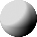
Figure 17-10 shows this material applied to a model of a sphere. (The sphere model itself is not shown because it contains several thousand triangles, and is therefore rather large.)

Figure 17-10. Sphere with DiffuseMaterial

SpecularMaterial

SpecularMaterial models a shiny surface. A SpecularMaterial shows highlights where it reflects the light source, and as with a real object, these highlights will shift as the point of view moves around. Example 17-6 shows a SpecularMaterial.

Example 17-6. SpecularMaterial

<SpecularMaterial SpecularPower="30" Brush="White" />

Figure 17-11 shows this material applied to the same sphere as in Figure 17-10. (Two highlights have appeared because this particular example scene contains two light sources.) This has been rendered onto a black background because the material would be invisible on a white background.

Figure 17-11. Sphere with SpecularMaterial

Figure 17-11 looks a little odd. This is because you would not normally use a SpecularMaterial in isolation. The material is designed to be used in a MaterialGroup in combination with other material types such as a DiffuseMaterial. The highlights provided by a SpecularMaterial are added onto whatever is underneath.

The way a SpecularMaterial combines with what is underneath is different from ordinary transparency. Normal transparent rendering in 2D graphics in WPF generates weighted averages of colors. But a SpecularMaterial is additive. For example, suppose a specular material’s brush is bright green—a color of #00FF00. Imagine it appears on top of something bright red (i.e., #FF0000); for example, it is part of a material group, on top of a red diffuse material. The resultant highlight will be the color you get when adding red to green: #FFFF00, which is yellow. This is a different result from the averaging used by ordinary semitransparent alpha blending. If you had a rectangle of color #FF0000 and then painted one on top of it with the color #00FF00 and an Opacity of 0.5, the outcome for this combination would be the average of the R, G, and B channels for those colors, #808000, which is a rather dull shade of brown.

If adding in the highlight takes any of the red, green, or blue color channels past 100 percent, they will simply be clipped at 100 percent. This causes the highlight to bleach out, a bit like an overexposed area of a photograph. This is why Figure 17-11 has been rendered on a black background—a white background is already at maximum brightness, and attempting to add highlights won’t make it any whiter.

As with the DiffuseMaterial, you can provide any 2D Brush object to determine the color or texture of the material. In addition, you can specify a SpecularPower. This determines how much the highlights are spread out. A low number results in a wide spread, and a high number results in a more tightly focused highlight.

Figure 17-12 shows the same sphere as Figure 17-11 twice, with different SpecularPower values. On the left, the low value of 5 has caused the two highlights to spread out so far that they have merged into one. On the right, the high value of 100 has caused the two highlights to become very small.

Figure 17-12. SpecularPower of 5 (left) and 100 (right)

Warning

Lighting calculations are performed on a per-point basis. If you choose a high specular power, meaning that the highlights should look small and focused, you will need a fairly detailed model for the highlights to look correct. The triangles that make up the surface need to be significantly smaller than the size of the specular highlights in order to avoid strange artifacts. The example on the righthand side of Figure 17-12 is pushing it a little—the highlights look a little uneven, even though the sphere model contains 4,000 facets and fills more than 400 KB of XAML.

EmissiveMaterial

Both DiffuseMaterial and SpecularMaterial require external light sources to be visible. If all your light is coming from one direction, these materials will look completely black on the shadow side. But an EmissiveMaterial is its own light source.

An emissive material contributes to the output in the same way as a specular material: it adds to whatever was behind it. However, whereas a specular material’s contribution is based on viewing angles and light positions, an emissive material is unaffected by the light sources in a scene—it always contributes evenly across the whole surface.

Tip

Although an EmissiveMaterial illuminates itself, it does not act as a light source to other objects in the same 3D model. Shaped light sources are computationally complex to render and are beyond the 3D capabilities offered by WPF. However, if you want to create a 3D object that looks like a light source, you can fake it by placing a light source in the scene at the same location.

Example 17-7 shows a simple EmissiveMaterial. In practice, you would not normally use as simple a brush as this. As Figure 17-13 shows, when this is applied to the same sphere as the earlier examples, it produces a rather dull result.

Example 17-7. EmissiveMaterial

<EmissiveMaterial x:Key="emissiveBlueMaterial" Brush="#00FFFF" />

As with the SpecularMaterial example, this figure has been rendered onto a black background—additive rendering onto white only ever results in white.

Figure 17-13. Sphere with EmissiveMaterial

In practice, an EmissiveMaterial would usually be used only with a more varied brush, such as an ImageBrush. Also, like a SpecularMaterial, it would typically be used as part of a MaterialGroup.

MaterialGroup

MaterialGroup allows multiple materials to be combined into a single material. For example, you might want to use a DiffuseMaterial to define the basic solid appearance, but provide a less dull finish by adding a SpecularMaterial. Example 17-8 shows such a material.

Example 17-8. Diffuse and specular materials in a MaterialGroup

<MaterialGroup>
  <DiffuseMaterial Brush="#00FFFF" />
  <SpecularMaterial SpecularPower="30" Brush="White" />
</MaterialGroup>

Figure 17-14 shows the results. Note that the diffuse material provides a complete solid basic finish for the shape to which the specular material can add highlights. We no longer need a black background to be able to see the highlights. This is the normal way to use a specular material.

Figure 17-14. Sphere with MaterialGroup

By combining with other materials in a MaterialGroup, EmissiveMaterial can play a more convincing role than the rather dull example in Figure 17-13. Figure 17-15 shows a sphere with a similar material group to that in Figure 17-14, but with an added EmissiveMaterial.

Figure 17-15. MaterialGroup with EmissiveMaterial (Figure F-27)

Notice how the text “glow” is visible and bright even though it runs into the part of the sphere that is in shadow. This is because it is rendered as an EmissiveMaterial and is therefore unaffected by the scene’s lighting. This illustrates EmissiveMaterial’s main purpose: to make areas of a shape “light up.” Example 17-9 shows the material for Figure 17-15.

Example 17-9. MaterialGroup with EmissiveMaterial

<MaterialGroup>
  <DiffuseMaterial Brush="#0000FF" />
  <SpecularMaterial SpecularPower="30" Brush="White" />
  <EmissiveMaterial>
    <EmissiveMaterial.Brush>
      <VisualBrush ViewboxUnits="Absolute" Viewbox="0,0,150,50">
        <VisualBrush.Transform>
          <TransformGroup>
            <TranslateTransform X="0.35" Y="0.5" />
          </TransformGroup>
        </VisualBrush.Transform>
        <VisualBrush.Visual>
          <Grid Width="150" Height="50">
            <TextBlock FontSize="8" Text="Glow!" Foreground="#ff80a0"
                       HorizontalAlignment="Center">
              <TextBlock.BitmapEffect>
                <OuterGlowBitmapEffect GlowColor="#ff8000" GlowSize="1" />
              </TextBlock.BitmapEffect>
            </TextBlock>
          </Grid>
        </VisualBrush.Visual>
      </VisualBrush>
    </EmissiveMaterial.Brush>
  </EmissiveMaterial>
</MaterialGroup>

Now that we have seen how to define materials, we can finally complete the GeometryModel3D we started building earlier. Example 17-10 shows the full model item, with both a geometry and a material.

Example 17-10. Complete GeometryModel3D

<GeometryModel3D>
  <GeometryModel3D.Geometry>
    <MeshGeometry3D Positions="0,1,0  1,−1,0  −1,−1,0"
                    Normals="0,0,1  0,0,1  0,0,1"
                    TriangleIndices="0,2,1" />
  </GeometryModel3D.Geometry>

  <GeometryModel3D.Material>
    <DiffuseMaterial Brush="Red" />
  </GeometryModel3D.Material>

  <GeometryModel3D.BackMaterial>
    <DiffuseMaterial Brush="Green" />
  </GeometryModel3D.BackMaterial>
</GeometryModel3D>

Notice that we’ve added two materials, one for the front and one for the back. This is because our shape is open, so the surface can be seen from either side. Some shapes, such as a sphere, are closed, so only one side of the mesh will ever be visible (assuming you don’t move the camera into and out of the shape). For such shapes, you would supply just a single material.

Now that have a complete model, we need to connect this into the Viewport3D. However, we can’t connect it in directly—there’s one more step.

ModelVisual3D

The various classes derived from Model3D that make up our model are just a description of the scene. They are in many ways analogous to the elements that make up a Drawing in the 2D world: both are descriptions of visual content; both are shareable objects that derive from Freezable^[115] and neither can render something on-screen of its own accord.

A Drawing needs to be connected to some kind of Visual object to be rendered and to enable input handling. Likewise, a Model3D needs to be connected to a ModelVisual3D in order to be rendered and to support hit testing.

Tip

ModelVisual3D does not derive from Visual. It derives from Visual3D instead. However, it does form part of the visual tree. If you use the VisualTreeHelper class to navigate the tree, it reports both kinds of elements. We described VisualTreeHelper in Chapter 9.

Example 17-11 brings together the various other pieces we’ve looked at so far to form a complete, if rather simple, example. This adds the completed GeometryModel3D from Example 17-10 to the Model3DGroup in Example 17-2. This Model3DGroup provides the Content of a ModelVisual3D. This in turn is the child of a Viewport3D, which lets us host this 3D content in a 2D WPF user interface. Finally, in order to describe the point of view from which we would like to render the scene, we have added the PerspectiveCamera from Example 17-1.

Example 17-11. Complete 3D example

<Viewport3D>
  <Viewport3D.Camera>
    <PerspectiveCamera Position="0,0,10" LookDirection="0,0,−1"
                       UpDirection="0,1,0" FieldOfView="45" />
  </Viewport3D.Camera>

  <ModelVisual3D>
    <ModelVisual3D.Content>
      <Model3DGroup>

        <DirectionalLight Direction="0,0,−1" />

        <GeometryModel3D>
          <GeometryModel3D.Geometry>
            <MeshGeometry3D Positions="0,1,0  1,−1,0  −1,−1,0"
                            Normals="0,0,1  0,0,1  0,0,1"
                            TriangleIndices="0,2,1" />
          </GeometryModel3D.Geometry>

          <GeometryModel3D.Material>
            <DiffuseMaterial Brush="Red" />
          </GeometryModel3D.Material>

          <GeometryModel3D.BackMaterial>
            <DiffuseMaterial Brush="Green" />
          </GeometryModel3D.BackMaterial>
        </GeometryModel3D>

      </Model3DGroup>
    </ModelVisual3D.Content>
  </ModelVisual3D>
</Viewport3D>

For all our efforts, we might have expected something slightly more impressive than the result shown in Figure 17-16. But remember, we did set out to create the simplest possible MeshGeometry3D, so we cannot be too surprised at the modest results.

Figure 17-16. Rendered 3D content

Creating 3D shapes by typing in mesh data is a slow and awkward process. In practice, most 3D models will be designed in interactive modeling applications or generated by code. However, Figure 17-16 is so flat that before moving on, we should at least tweak the model so that it looks like it’s three-dimensional. Example 17-12 shows modified versions of the camera and mesh.

Example 17-12. Tweaking the model

<PerspectiveCamera Position="−4,1,10" LookDirection="4,−1,−10"
                   UpDirection="0,1,0" FieldOfView="45" />
...
<MeshGeometry3D Positions="0,1,0  1,−1,1  −1,−1,1  1,−1,−1  −1,−1,−1"
                Normals="0,1,0  −1,0,1  1,0,1  −1,0,−1  1,0,−1"
                TriangleIndices="0,2,1  0,3,1  0,3,4  0,2,4" />

Figure 17-17 shows the resulting tetrahedron. To make the faces more visually distinctive, alternate faces in the model have been turned backward by reversing the index order in TriangleIndices. So, the front face in this example is red, but the face visible on the side is green—the color of the back material. (Although this is a convenient hack for making the faces stand out, it has the unfortunate side effect of inverting the lighting calculations for those faces, so the shading looks inconsistent. In practice, if you want different faces of your model to have different materials, using multiple Geometry3D objects would be a better technique.)

Figure 17-17. Visibly three-dimensional content

We have now examined the core types at the heart of WPF’s 3D API. As you’ve seen, many of these are analogous to WPF’s 2D types. Table 17-1 summarizes the similarities between these types. (For completeness, the table also contains a type we have not covered yet: Transform3D, which we will describe later.)

Table 17-1. Analogous 3D and 2D types

3D type	2D equivalent	Purpose
Visual3D	Visual	Abstract base class for elements in the visual tree
ModelVisual3D	Canvas	A visual element that can contain a group of visual elements
Model3D	Drawing	Abstract base class for model or drawing parts
GeometryModel3D	GeometryDrawing	A shape plus a material or brush (part of a model or drawing)
Model3DGroup	DrawingGroup	A collection of model or drawing parts
Geometry3D	Geometry	Abstract base class for shapes
MeshGeometry3D	PathGeometry	A shape
Material	Brush	Abstract base of classes describing how to paint a shape
Transform3D	Transform	Abstract base class of transformations such as scaling or rotation

Now that we’ve looked at the basics, it’s time to look at a few of the ways we can enhance the appearance of our 3D visuals. We’ll start by looking at the various kinds of light sources.

A 3D model can incorporate any number of light sources. It should include at least one so that you are able to see the objects in the model. In practice, you might want to add a few—a single light source can produce a somewhat stark appearance. WPF offers four different kinds of light.

AmbientLight

The simplest light source is AmbientLight. This provides an even illumination of all objects in the scene regardless of their location or orientation. Example 17-13 shows an AmbientLight.

Example 17-13. AmbientLight

<AmbientLight Color="White" />

The only property to set on an ambient light is Color. This property is present on all lights, and it indicates the color of the light emitted by the source. Note that the Color property determines not just the color of illumination, but also the intensity—White is the brightest color; a darker color such as Gray will provide less illumination. Figure 17-18 shows the results. This makes it clear that you would not normally use an AmbientLight as your only source of illumination. The sphere rendered in this example is the same one shown in Figure 17-14, but in that earlier figure, we could see reflected highlights and shadows thanks to the SpecularMaterial and DiffuseMaterial in the object’s material group. The same material is in use here, but because AmbientLight illuminates the scene in a completely uniform way, the sphere looks flat.

Figure 17-18. Ambient lighting

You would not normally use an AmbientLight in isolation like this unless your goal was to create an exaggeratedly artificial look. AmbientLight is designed to be used in conjunction with some directional or positional light sources. The other sources would provide most of the light, with a dim AmbientLight ensuring that any parts of the model in shadow are not plunged into complete darkness.

DirectionalLight

DirectionalLight provides a slightly more natural form of illumination. It models a bright distant light source such as the sun. So, you do not specify a position for DirectionalLight, you merely configure the direction from which it illuminates, as Example 17-14 shows. The light in this example arrives from behind and slightly above the viewer. (This assumes that the camera is positioned so that a positive y direction means up, and positive z means toward the viewer.)

Example 17-14. DirectionalLight

<DirectionalLight Color="White" Direction="0,−1,−0.5" />

Figure 17-19 shows the same sphere as Figure 17-18, but illuminated with this directional light. As you can see, the materials are now able to do their job. The upper half is brighter than the lower half thanks to the diffuse material, and there is a reflective highlight from the specular material. These effects reveal the curvature of the surface.

Figure 17-19. Directional lighting

Tip

Although the sphere clearly has a side that is in shadow, this is simply a result of how the DiffuseMaterial works: parts of the shape that face away from any light source will be painted dark, giving the appearance of a shadow. However, objects cannot cast shadows onto each other. For example, if we added a flat surface representing the ground to the model in Figure 17-19, it would not show a shadow of the sphere. This is because WPF uses a simple lighting model—each object’s illumination is calculated in isolation, so one object cannot cast a shadow on another.

PointLight

PointLight is useful for simulating a local light source, such as a lamp in a room. The relative position of a PointLight and an object has an impact on how the one illuminates the other. The simplest use of a PointLight involves setting its color and position, as shown in Example 17-15.

Example 17-15. PointLight

<PointLight Color="White" Position="0,1,1.5" />

Figure 17-20 shows the effect of this on a scene containing two spheres. The spheres are centered on the x-axis, at x positions of −0.6 and 0.6. This means the PointLight is slightly above and in front of the spheres, but horizontally centered between them. This positioning is evident in the shadows and highlights on the spheres—the highlights point toward the position of the PointLight.

Figure 17-20. Point lighting

If you were to animate the position of the light, the highlights would follow the light around. Figure 17-21 shows the same scene with the Position of the PointLight changed to 4, −2, 1.5.

Figure 17-21. Moving a point light

Real light sources provide more illumination when they are nearby than when they are distant. By default, a PointLight does not behave this way—a very distant PointLight illuminates just as brightly as a nearby one. However, you can configure it to attenuate the brightness over distance in order to model a real light source more realistically.

Attenuation of a PointLight is calculated as a quadratic function of distance (i.e., a function with three terms: the square of the distance, the distance itself, and a constant). This is designed to correspond to how light sources attenuate naturally. Two factors contribute to how real light sources diminish with distance.

The first factor is that light spreads out. For example, put a light in a small room with dimensions of 10×10×10 feet. The area of each wall is 100 square feet, so including the floor and ceiling as well as the walls, the light has to illuminate a total surface area of 600 square feet. Now put the same light in a larger room with dimensions of 30×30×30 feet. Each wall is now 900 square feet, a total area of 5,400 square feet to illuminate. We increased the dimensions by a factor of 3, but the total area to be illuminated by our lamp went up by a factor of 9—the square of the change. Because it’s the same lamp, it’ll be giving out just as much light as before, but as this light is spread over an area nine times larger, the walls would appear nine times darker.

You can model this by setting the QuadraticAttenuation property—this sets the multiplier for the square term of the attenuation equation. Figure 17-22 shows the effect of this. The two spheres’ centers are 1.6 units apart, and the light source is just to the right of the rightmost sphere. The QuadraticAttenuation has been set to 0.2, and as you can see, this causes the left sphere to be darker than the right sphere.

Figure 17-22. Attenuation

The second cause of natural attenuation is dust and other small airborne obstacles. These gradually diminish the intensity of light over distance. The effect of this is proportional to the distance the light has traveled—the farther it has to go, the more stuff gets in its way. You can model this by setting the LinearAttenuation property.

There is a third term for the attenuation equation, set by the ConstantAttenuation property. By default, this is set to 1, and the other two attenuation properties default to 0. This ensures that the level of attenuation is constant by default. (A sum total attenuation of 1 means no attenuation—only values higher than 1 will cause attenuation to occur.)

Warning

PointLight is more expensive than either AmbientLight or DirectionalLight, because it requires more complex lighting calculations. If you have more than a handful of such lights and you encounter performance problems with 3D content, try reducing the number of point lights. The same applies to the SpotLight described in the next section.

SpotLight

SpotLight is very similar to PointLight—it supports all the same properties. However, whereas a PointLight casts light in all directions, a SpotLight casts a cone of light in a specific direction. You specify the direction with the Direction property. You set the width of the cone with InnerConeAngle and OuterConeAngle properties. Everything inside InnerConeAngle is fully illuminated, and then the degree of illumination fades to nothing by the time the OuterConeAngle is reached. Example 17-16 shows a SpotLight.

Example 17-16. SpotLight

<SpotLight Color="White" Position="−2,2,6" Direction="2,−2,−6"
           InnerConeAngle="8" OuterConeAngle="12" />

Figure 17-23 shows the result. As you can see, only a circular region to the upper left of the sphere has been illuminated. The rest falls outside of the OuterConeAngle, so it is in darkness.

Figure 17-23. SpotLight

Remember that WPF performs illumination calculations on a per-point basis. So if you take a surface that contains very few points, and you shine a spotlight onto the surface expecting to see a spot appear, you will be disappointed. Figure 17-24 illustrates this. Both of the images are of a simple flat square surface. Both surfaces have the same material and have been lit with the same spotlight from the same angle. The two models are identical in every respect except one: the surface on the left has been subdivided into a 64×64 grid of evenly spaced points, whereas the surface on the right is defined by just the four corner points. Figure 17-25 gives an impression of the difference between the two models—it shows the outlines of the triangles that make up the two squares. (In fact, the model on the left of Figure 17-25 is only a 16× 16 grid—Figure 17-24 has been subdivided into pieces one-quarter the height and width. However, those would have been too small to see what’s going on.)

Figure 17-24. Impact of point density on illumination

Figure 17-25. Highly tessellated square (left) and four-point square (right)

Geometrically speaking, the two surfaces have exactly the same shape: the grid of points making up the first surface lies in the same plane and within the same bounds. But as you can see, the two look very different. The surface on the left has sufficiently densely packed points that you can easily make out the shape of the spot cast by the SpotLight. With the shape on the right, however, only four lighting calculations have been performed—one for each corner—and the results have been interpolated across the shape, so the result is just a gradual color fade to one corner. (If we point the spotlight directly in the middle of the surface on the right, it remains completely black, because none of the four points falls inside the spotlight’s cone.)

Although you need a fairly dense mesh for detailed lighting effects to work, you might be able to achieve a similar effect using materials instead. Rather than using a spotlight to project a spot onto a surface, you could use an EmissiveMaterial in conjunction with a suitable brush texture. Texture mapping does not require a high point density to work correctly, as you’re about to see.

Because DiffuseMaterial, SpecularMaterial, and EmissiveMaterial are based on brushes, we need not be limited to plain colors for our surfaces. We are free to paint 3D objects with gradient brushes, bitmaps, or drawings. We can even use any part of a user interface as a brush with which to paint a 3D object. An image or pattern used to paint a 3D surface is often referred to as a texture.

To use a textured material, we must tell WPF exactly how the brush should be positioned on the surface. With a solid color, this is a nonissue—the entire surface is of uniform color. But with a bitmap, we need to specify exactly where the image is projected onto the surface.

MeshGeometry3D provides the TextureCoordinates property for exactly this purpose. For each 3D point in the Positions, you can specify a 2D texture coordinate. Example 17-17 defines a simple square surface with four points, joined together with two triangles.

<MeshGeometry3D Positions="−1,1,0  1,1,0  −1,−1,0,  1,−1,0"
                Normals="0,0,1  0,0,1  0,0,1  0,0,1"
                TextureCoordinates="0,0  1,0  0,1  1,1"
                TriangleIndices="0,2,3  0,3,1" />

Figure 17-26 shows the texture coordinates specified for each corner of the square, and how the TriangleIndices collection joins these together with triangles. Texture coordinates are specified in the coordinate space of the brush’s Viewport. As we saw in Chapter 13, by default tile brushes use a mapping mode of RelativeToBoundingBox, which means that their viewport ranges from 0,0 to 1,1. So, the texture coordinates in Example 17-17 tell the brush to fill the surface area completely.

Figure 17-26. Texture coordinate positions

With the texture coordinates specified, we can now use any tile brush to form the material for this shape. Example 17-18 uses an ImageBrush to paint the surface with a bitmap.

<GeometryModel3D>
  <GeometryModel3D.Geometry>
    <MeshGeometry3D Positions="−1,1,0  1,1,0  −1,−1,0, 1,−1,0"
                    Normals="0,0,1  0,0,1  0,0,1 0,0,1"
                    TextureCoordinates="0,0 1,0 0,1 1,1"
                    TriangleIndices="0,2,3 0,3,1" />
  </GeometryModel3D.Geometry>

  <GeometryModel3D.Material>
    <DiffuseMaterial>
      <DiffuseMaterial.Brush>
        <ImageBrush ImageSource="MyImage.jpg" />
      </DiffuseMaterial.Brush>
    </DiffuseMaterial>
  </GeometryModel3D.Material>
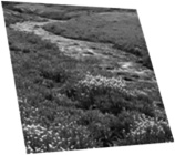
</GeometryModel3D>

Figure 17-27 shows the results.

Figure 17-27. Material with ImageBrush

Alternatively, you could paint the surface with a video by using the Material in Example 17-19.

<DiffuseMaterial>
  <DiffuseMaterial.Brush>
    <VisualBrush>
      <VisualBrush.Visual>
        <MediaElement Source="MyVideo.wmv" />
      </VisualBrush.Visual>
    </VisualBrush>
  </DiffuseMaterial.Brush>
</DiffuseMaterial>

This example uses a VisualBrush to create a material based on a MediaElement. We can use the same brush type with any UI element. For example, we could map a whole 2D UI onto a 3D surface. Figure 17-28 shows an ordinary data entry UI mapped onto our simple square surface and viewed from an angle.

Figure 17-28. 2D UI mapped onto a 3D surface

Although this technique makes for nifty-looking demos, it has a fundamental limitation: you cannot click on any of the controls on the 3D surface. VisualBrush lets us paint 2D or 3D elements with the contents of a visual, but it only lets us create an image. It does not provide a built-in way to route mouse input aimed at the surface back to the original visual. The user interface in this example is strictly a “look but don’t touch” affair.

Just as you can apply a transform to any 2D element in WPF, you can also transform any ModelVisual3D, or any of the types derived from Model3D. The set of transforms is much the same—you can rotate, scale, shear, or translate any part of the 3D model. However, to effect these operations in three dimensions requires slightly more information than it does in two dimensions, so we cannot simply use the 2D transform classes in 3D. WPF therefore defines a set of 3D transform types, all of which derive from the abstract Transform3D class.

<ModelVisual3D Content="{StaticResource cylinderModel}">
  <ModelVisual3D.Transform>
    <TranslateTransform3D OffsetX="−1" OffsetZ="0" />
  </ModelVisual3D.Transform>
</ModelVisual3D>
<ModelVisual3D Content="{StaticResource cylinderModel}">
  <ModelVisual3D.Transform>
    <TranslateTransform3D OffsetX="−0.5" OffsetZ="−0.5" />
  </ModelVisual3D.Transform>
</ModelVisual3D>
<ModelVisual3D Content="{StaticResource cylinderModel}">
  <ModelVisual3D.Transform>
    <TranslateTransform3D OffsetX="0" OffsetZ="−1" />
  </ModelVisual3D.Transform>
</ModelVisual3D>
<ModelVisual3D Content="{StaticResource cylinderModel}">
  <ModelVisual3D.Transform>
    <TranslateTransform3D OffsetX="0.5" OffsetZ="−1.5" />
  </ModelVisual3D.Transform>
</ModelVisual3D>
<ModelVisual3D Content="{StaticResource cylinderModel}">
  <ModelVisual3D.Transform>
    <TranslateTransform3D OffsetX="1" OffsetZ="−2" />
  </ModelVisual3D.Transform>
</ModelVisual3D>

ScaleTransform3D

A ScaleTransform3D enlarges or reduces an object. The scale factors are specified independently for each dimension with the ScaleX, ScaleY, and ScaleZ properties. There are also three properties to specify the center of scaling: CenterX, CenterY, and CenterZ. (The center of scaling is the point that remains in the same place before and after the scale operation.)

Example 17-21 uses a ScaleTransform3D to display a model stretched to double its normal width and depth, and one-quarter its normal height. This will use the default scale center of 0,0,0.

Example 17-21. ScaleTransform3D

<ModelVisual3D Content="{StaticResource cylinderModel}">
  <ModelVisual3D.Transform>
    <ScaleTransform3D ScaleX="2" ScaleY="0.25" ScaleZ="2" />
  </ModelVisual3D.Transform>
</ModelVisual3D>

Figure 17-29 shows the results. This is the same cylinder model as used for Figure 17-1, but the scaling has made it look shorter and squatter.

Figure 17-29. ScaleTransform3D

RotateTransform3D

RotateTransform3D allows objects to be rotated. Two pieces of information are required: the angle of rotation and the axis around which to rotate. Example 17-22 rotates a model by 45 degrees around the x-axis. WPF follows the usual mathematical convention that a positive angle indicates a counterclockwise rotation.

Example 17-22. Rotation around the x-axis

<ModelVisual3D Content="{StaticResource cylinderModel}">
  <ModelVisual3D.Transform>
    <RotateTransform3D>
      <RotateTransform3D.Rotation>
        <AxisAngleRotation3D Axis="1,0,0" Angle="45" />
      </RotateTransform3D.Rotation>
    </RotateTransform3D>
  </ModelVisual3D.Transform>
</ModelVisual3D>

Figure 17-30 shows the original unrotated model on the left. In the center is the model as rotated by Example 17-22. The righthand side shows how the model would look if rotated around the z-axis (i.e., if the Axis property had been set to 0,0,1). Rotation around the y-axis is not shown, because this particular model has rotational symmetry about that axis, so there would be no visible difference. (If the object had a bitmap texture material instead of a plain color, such a rotation would have a visible effect.)

Figure 17-30. 2D Rotation

Many 3D graphics systems use quaternions to represent rotations. A quaternion is a number with four components, and there are some standard rules for how to perform mathematical operations on quaternions. There is also a widely adopted system for encoding a 3D rotation into a quaternion.^[116] Example 17-23 shows how to apply a rotation expressed as a quaternion. This particular quaternion happens to correspond to a rotation of 120 degrees around the axis −1,1,1.

Example 17-23. QuaternionRotation

<RotateTransform3D>
  <RotateTransform3D.Rotation>
    <QuaternionRotation3D Quaternion="−0.5,0.5,0.5,0.5" />
  </RotateTransform3D.Rotation>
</RotateTransform3D>

The relationship between the numbers in a quaternion and the resultant rotation is somewhat opaque compared to the AxisAngleRotation3D representation. However, there are two useful characteristics of quaternions that explain their ubiquity in 3D graphics systems. First, it is easy to concatenate multiple rotations—you can simply multiply two quaternions together, and the result is a quaternion that represents the combined rotations. Second, there is a fairly straightforward way of interpolating between two quaternions that guarantees to offer the shortest transition between any two rotations. Without quaternions, this is not always straightforward if the two rotations are around different axes.

RotateTransform3D therefore accepts for the Rotation property either an AxisAngleRotation3D or a QuaternianRotation3D. WPF defines a Quaternion structure to represent a quaternion. This supports interpolation between two quaternions with its Slerp method. (Slerp is short for Spherical Linear intERPolation.) The QuaternionAnimation class also uses this interpolation method to animate between two rotations.

<Transform3DGroup>
  <ScaleTransform3D ScaleX="2" ScaleY="2" />
  <TranslateTransform3D OffsetX="1" OffsetZ="−2" />
</Transform3DGroup>

<MatrixTransform3D Matrix="−1,0,0,0
                            0,1,0,0
                            0,0,1,0
                            0,0,0,1" />

You can represent some kinds of data as a three-dimensional graph. For example, certain mathematical functions can be visualized this way. So can some sets of physical measurements (e.g., height information from map data). Figure 1-21 shows an example.

Figure 17-31. 3D plot of data (Figure F-2)

To display data in this form, you need to write code that will generate a mesh from the data. Let’s look at an example that creates the MeshGeometry3D shown in Figure 1-21 from a two-dimensional array of floating-point numbers. To be able to display a 3D model, we will of course need a Viewport3D. Example 17-26 shows the XAML for a window containing a Viewport3D with a camera and some light sources.

<Window x:Class="Generate3DMesh.Window1"
    xmlns="http://schemas.microsoft.com/winfx/2006/xaml/presentation"
    xmlns:x="http://schemas.microsoft.com/winfx/2006/xaml"
    Title="Generate3DMesh" Height="400" Width="400">

    <Grid x:Name="mainGrid">
      <Viewport3D x:Name="vp">
        <Viewport3D.Camera>
          <PerspectiveCamera Position="5,4,6" LookDirection="−5,−3.75,−6"
                             UpDirection="0,1,0" FieldOfView="10" />
        </Viewport3D.Camera>

        <ModelVisual3D>
          <ModelVisual3D.Content>
            <Model3DGroup>
              <AmbientLight Color="#222" />
              <DirectionalLight Color="#aaa" Direction="−1,−1,−1" />
              <DirectionalLight Color="#aaa" Direction="1,−1,−1" />
            </Model3DGroup>
          </ModelVisual3D.Content>

          <ModelVisual3D x:Name="modelHost" />

        </ModelVisual3D>
      </Viewport3D>
    </Grid>
</Window>

Notice that this example contains an empty ModelVisual3D element named modelHost. This is where we will add the 3D model that we build to represent the graph. Example 17-27 shows how the code-behind file initializes the window: it builds the data for the graph, builds a 3D model from the data, and then adds that model to the modelHost placeholder.

public partial class Window1 : Window {

    public Window1(  ) {
        InitializeComponent(  );

        double[,] points = GraphDataBuilder.BuildSincFunction(100, 100, 2.5, 5);
        ModelVisual3D vis3D = BuildModelVisual3DFromPoints(points);
        modelHost.Children.Add(vis3D);
    }
    ...
}

Example 17-28 shows the function that generates the data. It contains no 3D-specific code—it just builds a suitable two-dimensional array, using the mathematical sinc function, a popular function in signal processing applications that also happens to look good in 3D graphs. (.NET doesn’t provide a built-in implementation of sinc, so this code provides its own. The sinc function is defined to be sin(x)/x, except for when x is 0, where it is defined to be 1.)

class GraphDataBuilder {
    public static double[,] BuildSincFunction(int xPoints, int yPoints,
                                              double cycles, double height) {
        double[,] points = new double[xPoints, yPoints];
        for (int yIndex = 0; yIndex < yPoints; ++yIndex) {
            double y = yIndex; y /= ((yPoints − 1) / 2.0); y −= 1;
            for (int xIndex = 0; xIndex < xPoints; ++xIndex) {
                double x = xIndex; x /= ((xPoints − 1) / 2.0); x −= 1;

                double d = Math.Sqrt(x * x + y * y) * 2 * Math.PI * cycles;
                points[xIndex, yIndex] = (d == 0 ? 1 : Math.Sin(d) / d) * height;
            }
        }
        return points;
    }
}

After calling this BuildSincFunction method to generate the data, Example 17-27 calls the BuildModelVisual3DFromPoints method shown in Example 17-29 to convert this into a ModelVisual3D.

public partial class Window1 : Window {
    ...
    static ModelVisual3D BuildModelVisual3DFromPoints(double[,] points) {
        MeshGeometry3D mesh = MeshBuilder.BuildMeshFromPoints(points, 1, 1);
        GeometryModel3D model = BuildModel3DFromMesh(mesh);
        ModelVisual3D vis3D = new ModelVisual3D(  );
        vis3D.Content = model;
        return vis3D;
    }

The structure of this method reflects the structure of elements we need to create in order to build a complete 3D model. We need a mesh to represent the shape of the surface. This must be connected to a GeometryModel3D in order to define the materials for the surface. This model is then wrapped in a ModelVisual3D, allowing the InitializeComponent method in Example 17-27 to add it to the 3D visual tree.

Example 17-29 calls a helper method to build the mesh: BuildMeshFromPoints. This is shown in Example 17-30.

class MeshBuilder {
    public static MeshGeometry3D BuildMeshFromPoints(double[,] data,
                        double textureWidth, double textureHeight) {
        Point3DCollection points;
        PointCollection textureCoordinates;
        Int32Collection triangleIndices;
        BuildMeshData(data, textureWidth, textureHeight,
                   out points, out textureCoordinates, out triangleIndices);
        points.Freeze(  );
        textureCoordinates.Freeze(  );
        triangleIndices.Freeze(  );

        MeshGeometry3D mesh = new MeshGeometry3D(  );
        mesh.Positions = points;
        mesh.TextureCoordinates = textureCoordinates;
        mesh.TriangleIndices = triangleIndices;

        return mesh;
    }
    ...
}

This assembles the constituent parts of a MeshGeometry3D—the points and triangle indices defining the surface shape, and the texture coordinates that define how a texture is mapped onto the surface. Notice that this code freezes the collections containing the data. Calling Freeze tells WPF that we will not be changing any of these collections again. This enables it to handle the data more efficiently—it doesn’t need to do any of the housekeeping that would be necessary to be able to respond to changes to the data.

BuildMeshData, another helper function, shown in Example 17-31, performs all of the work of generating the mesh data.

class MeshBuilder {
    ...

    static void BuildMeshData(double[,] data,
                            double textureWidth, double textureHeight,
                            out Point3DCollection points,
                            out PointCollection textureCoordinates,
                            out Int32Collection triangleIndices) {

        // 1: initialization
        int width = data.GetLength(0);
        int height = data.GetLength(1);

        int pointCount = width * height;
        points = new Point3DCollection(pointCount);
        textureCoordinates = new PointCollection(pointCount);

        int triangleCount = 2 * (width - 1) * (height - 1);
        triangleIndices = new Int32Collection(3 * triangleCount);


        // 2: iteration
        for (int yDataIndex = 0; yDataIndex < height; ++yDataIndex) {
            double yProportion = yDataIndex; yProportion /= (height - 1);
            // Adding points from top to bottom.
            // In 3D up means increasing Y, but in
            // 2D 0 is at the top.
            double outY = 0.5 - yProportion;
            double textureY = textureHeight * yProportion;

            for (int xDataIndex = 0; xDataIndex < width; ++xDataIndex) {
                double xProportion = xDataIndex; xProportion /= (width - 1);
                double outX = xProportion - 0.5;
                double textureX = textureWidth * xProportion;


                // 3: adding points
                points.Add(new Point3D(outX, outY, data[xDataIndex, yDataIndex]));
                textureCoordinates.Add(new Point(textureX, textureY));


                // Add triangles for everything but the last row and column.
                if (xDataIndex < (width - 1) && yDataIndex < (height - 1)) {
                    int topLeftIndex = xDataIndex + yDataIndex * width;
                    int bottomLeftIndex = topLeftIndex + width;

                    triangleIndices.Add(bottomLeftIndex);
                    triangleIndices.Add(bottomLeftIndex + 1);
                    triangleIndices.Add(topLeftIndex);

                    triangleIndices.Add(bottomLeftIndex + 1);
                    triangleIndices.Add(topLeftIndex + 1);
                    triangleIndices.Add(topLeftIndex);
                }
            }
        }
    }
}

The function begins by working out how many points and triangles will be required in the mesh to present all the data in the array. It also allocates the various collections to hold the mesh data.

Next, we start the nested loops that will iterate over the point data in the two-dimensional input array—we do this with the two for loops in the part of Example 17-31 labeled “2: iteration.”

The xProportion and yProportion variables track how far we are through the data, expressed as a number from 0 to 1. We then calculate two coordinates. The outX and outY coordinates are in 3D space, and will range over a unit square centered on the origin. The textureX and textureY coordinates will be used to generate the TextureCoordinates entries, and will range over the texture size passed into the function. Note that these coordinate systems use different conventions. The 3D coordinates use the common convention that increasing values of y mean “up,” but the texture coordinates use the TileBrush convention that increasing y values mean “down.”

Finally, the inner part of the loop adds the points—this is the part of Example 17-31 labeled “3: add points.” It creates both a 3D point for the mesh’s Positions collection, and the corresponding 2D point for the TextureCoordinates collection. The latter enables us to use a textured material to paint the mesh, should we wish to.

The inner loop also generates the triangles that join the points to form the surface by adding entries to the triangleIndices collection. (We skip this for the final row and column of points, because those will already have been joined to triangles from the previous line and column.)

Our work is nearly done. The mesh data returned by BuildMeshData will be wrapped in a MeshGeometry3D by BuildMeshFromPoints. As we saw in Example 17-29, our BuildModelVisual3DFromPoints helper will then wrap this in a GeometryModel3D by calling another helper, BuildModel3DFromMesh, shown in Example 17-32.

public partial class Window1 : Window {
    ...
    private static GeometryModel3D BuildModel3DFromMesh(MeshGeometry3D mesh) {
        Material front = new DiffuseMaterial(Brushes.Red);
        GeometryModel3D model = new GeometryModel3D(mesh, front);
        model.BackMaterial = new DiffuseMaterial(Brushes.Green);
        return model;
    }
}

This adds red and green materials for the front and back of the surface. As we saw in Example 17-29, this will then be wrapped in a ModelVisual3D by the BuildModelVisual3DFromPoints helper function. And, as Example 17-27 showed, this is added to the modelHost placeholder defined in the XAML shown in Example 17-26, enabling our generated model to be displayed by the Viewport3D.

The normal WPF mouse events and properties work when the mouse is over a Viewport3D just like they do for any other UI element. The shapes of the elements in the model will be taken into account—if your scene has areas with nothing in it, the Viewport3D will effectively be transparent in those areas, and if you move the mouse over those, it will be considered to be over whatever is behind the Viewport3D rather than over the Viewport3D itself. But as long as the mouse is over some 3D object, all the usual mouse events will be reported.

Sometimes it is useful to know exactly which part of your 3D model the mouse is over. For example, in an application that displays the graph shown in Figure 1-21, you might want to display the exact coordinates and value for the point currently under the mouse. You can call the VisualTreeHelper.HitTest method to retrieve all the necessary information. You can pass in a 2D position relative to the Viewport3D (e.g., the current mouse location), as Example 17-33 shows.

public partial class Window1 : Window {
    ...
    void myViewport_MouseMove(object sender, MouseEventArgs e) {
        Point mousePos = e.GetPosition(vp);
        PointHitTestParameters hitParams = new PointHitTestParameters(mousePos);
        VisualTreeHelper.HitTest(vp, null, delegate (HitTestResult hr) {
            RayMeshGeometry3DHitTestResult rayHit = hr as
                   RayMeshGeometry3DHitTestResult;
            if (rayHit != null) {
                Debug.WriteLine(rayHit.PointHit);
            }
            return HitTestResultBehavior.Continue;
        }, hitParams);
    }
}

This shows an event handler for the MouseMove event of a Viewport3D. It uses the VisualTreeHelper class’s HitTest method in exactly the same way as you would for 2D hit testing. HitTest calls a callback method (the anonymous method in this example) for each item it finds at the specified position, and if one of the items is part of a 3D model, it will pass a RayMeshGeometry3DHitTestResult object as the parameter. This provides information about the item that was hit.

This particular example just prints the 3D location to the debugger by printing out the PointHit property. The result object also contains information about which Visual3D contained the model, and which Model3D and mesh were hit. It even tells you which triangle in the mesh was hit, and the position within that triangle. In the graph example, you can use this information to calculate the corresponding coordinates in the original graph data. Example 17-34 illustrates how to modify Example 17-33 to use this technique.

void myViewport_MouseMove(object sender, MouseEventArgs e) {
    Point mousePos = e.GetPosition(vp);
    PointHitTestParameters hitParams = new PointHitTestParameters(mousePos);
    VisualTreeHelper.HitTest(vp, null, delegate (HitTestResult hr) {
        RayMeshGeometry3DHitTestResult rayHit = hr as
               RayMeshGeometry3DHitTestResult;
        if (rayHit != null) {
            MeshGeometry3D mesh = rayHit.MeshHit as MeshGeometry3D;
            if (mesh != null) {
                int pointsWidth = points.GetLength(0);
                int y = rayHit.VertexIndex1 / pointsWidth;
                int x = rayHit.VertexIndex1 - (y * pointsWidth);

                Debug.WriteLine(string.Format("Point: {0},{1} value = {2}",
                    x, y, points[x, y]));
            }
        }
        return HitTestResultBehavior.Continue;
    }, hitParams);
}

This uses the RayMeshGeometry3DHitTestResult object’s VertexIndex1 property to discover which point in the mesh has been hit. It then works out which of the entries in the points array created in Example 17-31 this corresponds to.

The mouse will rarely be exactly over a vertex—it will usually be somewhere within the area of one of the mesh’s triangles. In this example, we don’t care about this because we’re just trying to correlate the mouse position back to one of the original data points, so we don’t need to know the exact location within the triangle. However, sometimes extra precision is necessary.

To enable you to work out the exact 3D position of the mouse, RayMeshGeometry3DHitTestResult provides a property for each corner of the triangle the mouse was over: VertexIndex1, VertexIndex2, and VertexIndex3. The relative position of the mouse within the triangle is indicated by the VertexWeight1, VertexWeight2, and VertexWeight3 properties. To calculate the exact position, you would calculate the sum of the three vertex positions, multiplied by the three weight properties, as shown in Example 17-35.

Point3D pointInMesh1 = mesh.Positions[rayHit.VertexIndex1];
Point3D pointInMesh2 = mesh.Positions[rayHit.VertexIndex2];
Point3D pointInMesh3 = mesh.Positions[rayHit.VertexIndex3];
double x = pointInMesh1.X * rayHit.VertexWeight1 +
           pointInMesh2.X * rayHit.VertexWeight2 +
           pointInMesh3.X * rayHit.VertexWeight3;
double y = pointInMesh1.Y * rayHit.VertexWeight1 +
           pointInMesh2.Y * rayHit.VertexWeight2 +
           pointInMesh3.Y * rayHit.VertexWeight3;
double z = pointInMesh1.Z * rayHit.VertexWeight1 +
           pointInMesh2.Z * rayHit.VertexWeight2 +
           pointInMesh3.Z * rayHit.VertexWeight3;

Point3D exactLocation = new Point3D(x, y, z);

The Viewport3D class allows you to add simple 3D models your user interface. The scene is built up with shapes defined by mesh geometries. These might be imported from a 3D modeling program, or generated at runtime from data. The appearance of the shapes is described by materials—combinations of 2D brushes and various lighting models. Because you can use any 2D brush, you can paint 3D surfaces with bitmaps, drawings, videos, or even a visual copy of a user interface. Finally, hit testing services enable you to find out with which part of a 3D model the user is interacting.