25

CAPITAL EXPENDITURE PLANS IN A RISKY WORLD

Decisions regarding long-term investment projects are referred to as capital budgeting decisions. In Chapter 6 we discussed how management of a firm should make capital budgeting decisions in a perfect capital market when future cash flows can be forecast with certainty. In this and the next chapter we consider projects with risky future cash flows. Such projects require that managers analyze the following factors:

• Each project's incremental future cash flows
• The probability distributions of these cash flows
• The present value of the cash flows, discounted according to the risks they present

In Chapter 6 we saw that a project's incremental cash flows comprise (1) operating cash flows (the change in the revenues, expenses, and taxes) and (2) investment cash flows (the acquisition and disposition of the project's assets). Given estimates of incremental cash flows for a project and an appropriate discount rate, we looked at alternative techniques to select the best of the available projects.

In deciding whether a project increases shareholder wealth, managers must weigh both its costs and its benefits. The costs are the cash flows necessary to create the project (the investment outlay) and the opportunity costs of not otherwise being able to use the cash tied up in the project. The benefits are the future cash flows expected to be generated by the project. But the future is unknown and therefore future cash flows are exposed to risk. As a result, management must evaluate the risk that cash flows will differ from their expected values. Risk and risk measurement were extensively discussed in Chapters 9 through 12, and the methods of those chapters will be applied here.

Risk arises from different sources, depending on environmental conditions, the industry in which the firm is operating, and the type of project being considered. Each of the following factors presents different sources of risk:

• Economic conditions. Will consumers be spending or saving? Will the economy be in a recession? Will the government stimulate spending? Will there be inflation?
• International conditions. Will the exchange rate between different countries’ currencies change? Are the governments of the countries in which the firm does business stable?
• Market conditions. Is the market competitive? How long does it take competitors to enter into the market? Are there any barriers, such as patents or trademarks, that will keep competitors away? Is there sufficient supply of raw materials and labor? How much will raw materials and labor cost in the future?
• Taxes. What will tax rates be in the future? Will Congress alter the tax system?
• Interest rates. What will be the cost of raising capital in future years?

Several further questions also arise. First, management must determine whether a new project's cash flow risks are the same as those of existing projects and if not, determine a suitable adjustment to the discount rate the company currently uses. The question of determining the project's optimal scale must also be resolved. These matters are discussed in Section 25.1. In Section 25.2 we show how, given a fixed operating plan, rates of return to projects are related to those of the entire firm. This matter is further discussed in Section 25.3, where it is related to the required rate of return on a tax saving generated by depreciation. In Section 25.4 we explore issues regarding multi-period planning of capital expenditure programs, and in Section 25.5 we deal with estimating cash flows and their risks in both single-period and multi-period contexts. Finally, in the next chapter we take a closer look at how the riskiness of a project is assessed.

25.1 A MARKET VALUE CRITERION

In a risky world with a perfect capital market, management can act in the best interests of stockholders without specific knowledge of their preferences because, as shown in Chapter 6, the only constraint on each consumer's decision is the present value of wealth. When there are no transactions costs, a risky cash flow stream's present value determines the consumer's opportunity set: The consumer is concerned with the project's present value rather than the details of the cash flows. For any expenditure profile having the same present value as the project's, cash flows can be rearranged without payment of charges other than interest, which of course entered into determining the value in the first place. Accordingly, the best that management can do for the firm's owners is to maximize the present value of their investments, and that present value is also the investment's market value.

In the context of capital budgeting under risk, a firm's managers can still implement the market value criterion by relating it to the firm's expected earnings and risk characteristics. The Capital Asset Pricing Model (CAPM) explained in Chapter 14 provides one theoretical framework¹ for how risky future cash flows can be evaluated, and we will use that framework here. Recall that, according to the CAPM, at equilibrium the expected return on securities of firm i is related to risk by:

where

Denote the distribution of project values at time 2 as V_i.² This distribution may itself be derived from the distributions of many future periods’ cash flows. If so, it is derived assuming the firm has an operating plan³ that will not change. Such a plan defines both the cash flow stream of the firm and its risk characteristics.

Let P_i represent the project's market value at time 1. We have:

Substituting the expression for E (r_i) from equation (25.2) into equation (25.1) and rearranging gives:

where cov(V_i, r_m) is the covariance between the value of the proposed firm at time 1 and the market portfolio return.

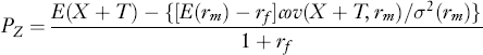
The numerator of the right-hand side of equation (25.3) is referred to as the time 2 certainty equivalent value of the cash flow V_i.⁴ Providing management knows the data on the right-hand side of equation (25.3), the market impact of a capital budgeting decision can be determined through assessment of its effects on cash flows. In other words, equation (25.3) gives management a means of determining whether or not a particular investment decision should be undertaken and if so, at what level.

The foregoing pricing equation can also be used to develop a risk-adjusted discount rate version of the CAPM. Recall that:

where β_i is the beta risk of firm i. We can then rewrite equation (25.3) in terms of beta risk as:

Then

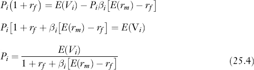
The numerator of equation (25.4) is equal to one plus the risk-adjusted rate of return required by the market. Subtracting one from the numerator gives the risk-adjusted rate of return:

equal to the risk-free rate plus a risk adjustment β_i[E(r_m) − r_f]. Note that the expected value of the cash flow stream is discounted in equation (25.4), whereas its certainty equivalent was discounted in equation (25.3).

Thus far, our framework has been formulated within a single-period setting. In a multi-period context, the risk-adjusted and certainty equivalent ways of determining value require careful treatment if they are to give equivalent results. These issues are discussed later in this chapter.

25.1.1 Basic Application to Capital Budgeting in a Risky World

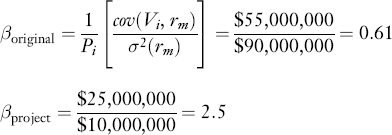
We now provide an example of how certainty equivalent values and risk-adjusted discount rates are used in capital budgeting under risk. Suppose a firm expects to generate E(V_i) = $100 million at time 2 from current operations, and that the firm has a time 1 market value of $90 million. The return on the market portfolio, E(r_m), is assumed to be 15% and the risk-free rate 5%, r_f. Hence,

[E(r_m) − r_f = 0.15 − 0.05 = 0.10

Suppose also that a new project available only in unit size and costing $6 million is contemplated. Further, suppose that the new project's expected cash flow one period later, denoted by E (F_i), is $13 million and that cov(F_i, r_m)/σ² (r_m) is $25 million. The foregoing numerical values are obtained under the assumption that the new project will be put to best use according to a fixed plan of operations that defines cash flows with the stated expected value and risk characteristics.

Should management undertake the new project? First, we can determine cov(V_i, r_m)/σ²(r_m) for the firm prior to adopting the new project. We do this by substituting the assumed numerical data into equation (25.3), which gives:

so that:

Now we may use the property of sums of random variables described in Web-Appendix L to write:

cov(V_i + F_i, r_m) = cov(V_i, r_m) + cov(F_i, r_m)

so that dividing the above equation by σ²(r_m) we get:

We just calculated the first ratio on the right-hand side of the above equation to be $55 million. We assumed that the second ratio is $25 million. Therefore,

The expected value of the firm with the new project is equal to:

E(V_i + F_i) = E(V_i) + (F_i)

Since it is assumed that E(V_i) is $100 million and E(F_i) is $13 million,

E(V_i + F_i) = $100,000,000 + $13,000,000 = $113,000,000

If the new project is undertaken, then the time 1 value of the total cash flow generated by the firm (exclusive of investment cost) will be, again using equation (25.3),

If the project is adopted, the market value of the firm is then expected to be $100 million. Recall that the market value prior to the adoption of the project was assumed to be $90 million. By adopting the project, the market value is expected to increase by $10 million. Thus, the $6 million investment cost would be more than compensated for, and the project should be undertaken.

The calculation can be put in another way to show that because the required rate of return on the project is less than its expected internal rate of return,⁵ the project has a positive present value to the firm. However, note first that the required rate of return on the new project is not equal to the firm's cost of funds before the project was undertaken. The rate of return required by the market, prior to the firm's adopting the project, is:

Subsequent to adopting the project, the required rate of return becomes:

Accordingly, the new project is not discounted by the market at 11.1%, but rather has a larger required rate of return, one that is in fact equal to 30%. To see this, note that the market value of the new project, using equation (25.3) to value it separately, is:

Then, since the new project creates expected cash flows of $13 million, the required rate of return⁶ on it is:

The same calculation can also be put another way. After the new project is adopted, the firm can be regarded as a portfolio of its old and new activities. In terms of market values, the new project accounts for 10% of the firm's activities, so we can stipulate that:

where x is an unknown rate of return on the new project. When solved, the foregoing expression gives x = 30%.

All the calculated rates of return are based on market values. Now since the new project can be implemented by the firm's existing owners for only $6 million, the internal rate of return on this $6 million investment must be in excess of the rate required by the marketplace, since the project's time 1 market value is $10 million. Nonetheless, if new investors were to purchase shares after the market value of the firm has changed to reflect the new project's adoption, they could earn only 13% on their investment, because the shares of the firm would be priced to yield just that expected return. The value created by the project would be retained by the original stockholders.

As a final point, we show that the firm's cost of capital can be calculated as a weighted average of market-required rates of return, with market values being used as weights. Let us calculate the β for the (combined) firm, and from that the overall required rate of return. We use the reasoning employed in obtaining (25.4). Thus:

Then using market values as weights, we obtain:

Finally, by equation (25.1) the required rate of return for the combined original firm and new project is:

0.05 + (0.15 − 0.05)(0.8) = 0:13 or 13%

We have assumed that the values of the firm and the project can be added to obtain the firm's new market value, an assumption that appears to ignore the possibility of synergy. However, this is not in fact the case. First, we can define any change in cash flows to be due to the project, because apart from adopting the project, output levels are assumed to be fixed. Moreover, since the level of the project itself is assumed to be fixed before the described calculations are made, the cash flows associated with the new project can indeed be added to the firm's preexisting cash flows (even if some of those newly created cash flows do result from synergistic effects).

The foregoing calculations establish several conclusions. First, the nature of the firm's business risk is determined by the investment projects it accepts. In the example, adopting the new project changes the firm's business risk, as reflected by the change in β and hence in the discount rate applied to the firm's total earnings stream. Second, management should adopt new projects when their internal rate of return exceeds the market-required rate of return for projects with a given measure of risk. Third, because of the possibility of different business risks, the required rate of return on a project is not necessarily the firm's prevailing cost of capital. (In the example it is a larger figure.) Fourth, adoption of a profitable project can alter the firm's overall cost of capital, because the risk of the firm's earnings stream can be altered by a new investment project.

25.2 COMPARING NEW AND EXISTING EARNINGS RISKS TO OBTAIN OPTIMAL CAPITAL EXPENDITURE PLANS

We can now use the CAPM to develop optimal capital budgeting rules similar to those discussed in Chapter 6. We consider first the case of projects yielding constant returns to scale, then the case of projects with diminishing returns.

25.2.1 Capital Expenditures with Constant Returns to Investment

Using the CAPM, let us consider the question of whether a new firm should be brought into being. As before, let V_i be the distribution of values of the proposed firm at time 2. The market value of the firm at time 1, P_i, can be determined using equation (25.3). Alternatively, the market-required rate of return for a firm's cash flows, E(r_j), can be found using equation (25.1).

Suppose that an initial investment of $75 million will be required to set up the new firm, no variation in the size of this investment being permissible. In other words, the optimal size of the investment is either zero or $75 million. Assume further that the distribution for (1) the cash flows to be generated, (2) the corresponding internal rate of returns for the firm (r_j,), and (3) the market portfolio return (r_m) is as follows:

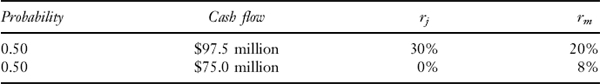
The estimation of these data is discussed in Section 25.5. From the estimated data, the following can be computed:

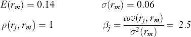
where ρ (r_j, r_m) is the correlation between the return on the proposed firm and the market portfolio.

Assume that the one-period risk-free rate (r_f) is 6%. Then applying equation (25.1) to the data, we find that the required rate of return for the proposed firm (i.e., the project) with the cash flow risk assumed is:

E(r_j) = r_f + β_j[E(r_m) − r_f = 0.06 + 2.5(0.08) = 0.25 = 25%

However, the proposed firm's expected internal rate of return (as computed from the distribution above) is only 15%, less than the market-required rate of return for an undertaking with the project's risk characteristics. In other words, the proposed firm should not be started because if it were brought into existence, the original investors could not sell the firm for a price as high as the cost of their investment.

The decision of whether an existing firm should adopt a project is a little more complex, as we now show. Suppose that a new project (not necessarily related to the one of the previous example) will expand the firm's time 2 distribution of values by a scale factor λ. Then, if V_i represents the original time 2 distribution of values, the new distribution is:

W_i = (1 + λ) V_i

It then follows immediately from equation (25.1) that the new time 1 value of the firm is Q_i =(1 + λ)P_i. It follows further that the market applies the same rate of discount to the augmented cash flows as it did to the original ones. The rate of discount after adopting the project is then:

the discount rate applied to the firm before the project was adopted. Accordingly, adopting new projects such that the firm's distribution of values changes only by a scale factor does not change the market-required rate of return. This situation is technically described as one of an investment yielding stochastically constant returns to scale.

Consequently, the rule for projects having the same business risk as the existing firm seems to be that such projects should be adopted, provided they can be implemented at a cost low enough to permit the project to earn at least the required rate of return. However, in this circumstance it is difficult to specify an optimal scale for the project unless one assumes either that the projects are available only in some limited amount or that the projects can only be implemented at increasing unit costs. Otherwise, if the adoption of any such project yields returns in excess of the return required by the marketplace, at what point does the firm's management stop investing in it?⁷

The difficulty lies in our assumption that cash flows expand by a scale factor, an assumption that really means constant internal rates of return are expected to be realized on all additional investments. Since this assumption is useful to illustrate the points developed above, but is at the same time unlikely to describe many practical situations, it will be worthwhile next to explore a scenario in which new project returns decline marginally.

25.2.2 Capital Expenditures with Diminishing Marginal Returns to Investment

To consider the case of diminishing marginal returns, suppose that funds invested at time 1 produce cash flows at time 2 according to:

where

Letting

α = [E(r_m) − r_f]/σ²(r_m)

the time 1 value of the cash flow Z (P_i) using equation (25.3) is:

Then equation (25.6) may be rewritten using equation (25.5) as:

as may be seen by applying the results from Web-Appendix L.

In this case the market value maximization objective can be expressed as maximizing the difference between value and investment cost, that is, P_i − I. The maximum occurs at an investment cost such that the time 2 internal rate of return falls to just 1 + r_f. To show this compactly, rewrite equation (25.7) as:

where γ = E(X) − cov(X, r_m), and consider:

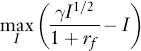
which has a solution given by:

FIGURE 25.1 OPTIMAL INVESTMENT DECISION IN A RISKY WORLD

Equation (25.8) is found by differentiating the equation on the previous line with respect to I and setting the result equal to zero. The left-hand term of equation (25.8) equals 1 + r_f, while the right-hand side is the slope of the market opportunity line for risk-free investments. Thus, when marginal returns to investment diminish, we have obtained a result similar to that in a risk-free situation: Management should invest up to the point where the certainty equivalent marginal internal rate of return equals the risk-free rate of interest. In this form, the situation may be depicted as in Figure 25.1.

The result may also be viewed as showing that at the optimum the expected rate of return on marginal investments is just equal to the rate the market requires for investments having that kind of business risk. To see the result in this manner, rewrite equation (25.8) as:

which can then be manipulated to yield:

That is, the marginal internal rate of return on an invested dollar—the left-hand side of equation (25.9)—equals the marginal rate of return required by the marketplace—the right-hand side of the equation—for cash flows having the risk characteristic indicated by the bracketed part of the second term on the right-hand side of the equation. Accordingly, we see that the rules for capital budgeting in a risky world are (loosely speaking) risk-adjusted analogs of the rules found in Chapter 6. That is, management should raise funds for projects until the marginal internal rate of return on the projects falls to where it equals the rate of interest required by the market.

As we have shown by drawing the transformation curve of Figure 25.1 in certainty equivalent terms that may be related to the market opportunity line for risk-free investments, the introduction of risk does not essentially change the conclusions obtained in Chapter 6. Alternatively, we have shown that the marginal internal rate of return for optimal amounts of investment will be equated to the market-required rate of return. Later in this chapter we shall show that while similar results are obtained for multi-period analyses, they require careful interpretation if erroneous conclusions are to be avoided.

25.3 REQUIRED RATES OF RETURN: FIRM, DIVISION, AND PROJECT

In the previous section we showed how the required rate of return on a firm's cash flows could be established, at varying output levels, with the aid of the CAPM. Providing we are now willing to specialize our assumptions by holding output levels fixed, the same approach can be used to relate rates of return on different projects, both to each other and to the market-required rate of return. (The reason for assuming fixed output levels will be discussed shortly.)

We next show that with fixed output levels the firm can be regarded as a portfolio of investment projects. Recalling equation (25.1), if we let the individual projects be defined by the index k, then we can write:

where

This approach shows that the return on the firm is the weighted average of the returns required by the market on each of the individual projects. The details are usefully explored with the aid of an example.

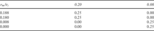
Consider the case of buying, at market value, a single steer. Suppose there are two revenue-producing activities: producing beef (project b) and producing hide (project h), which we assume generate statistically independent returns. We assume the cost of the steer is $450 and the variable cost of hide production is an additional $50. Moreover, we suppose that the amounts and returns to the two activities are as follows:

The returns are calculated on an investment cost basis, but as it will later turn out, investment cost equals market value for the assumed data. Therefore, the returns in this example can also be interpreted as those required by the market. The returns are uncorrelated according to:

ρ(r_h, r_m) = 0 and ρ(r_h, r_b) = 0

where the indices b, h, and m refer to producing beef or hide and to the market portfolio.

Combining the two activities’ returns while recalling their statistical independence, the distribution of returns from investing in the animal, which we denote by r_c, is as follows: 0.188, 0.180, 0.008, and 0, where each outcome has a probability of 1/4. From this distribution, the expected return from investing in the animal, E(r_c), is equal to 0.094. In order to apply the CAPM, we need more data. We will assume that r_m has two possible outcomes, 0.20 and 0 with equal probability. Then we know that:

E(r_m) = 0.10 and σ(r_m) = 0.010

And we will assume that r_f = 0.04.

Also suppose that returns on beef production and on the market portfolio are perfectly positively correlated [i.e., ρ(r_b, r_m) = 1]. We first apply the CAPM to investing with a view to carrying out both hide and beef production. For this purpose we prepare a table of joint probabilities using the previously stated data as shown below:

Then from the table we can calculate, using the definitions from Web-Appendix L,

E(r_c, r_m) = 0.0184 and E(r_c) E(r_m) = 0.0094

so that:

E(r_c, r_m) − E(r_c)E(r_m) = cov(r_c, r_m) = 0.0090

Therefore, using the calculated covariance in equation (25.1),

so the required rate of return just equals the expected rate of return we calculated earlier.

Calculation of the required rate of return on the hide production activity means determining E(r_h) according to equation (25.1). Remember ρ(r_h, r_m) = 0 so that cov (r_h, r_m) = 0. Consequently,

E(r_h) = r_f = 0.04

Finally, the required rate of return for the beef-producing activity is:

since ρ(r_b, r_m) = 1, so that:

cov(r_b, r_m) = σ(r_b)σ(r_m) = 0.10(0.10)

Now observe that the return on the combined activity is the weighted average of returns on the individual activities; that is,

where the weights are computed using the market values of the individual activities. In other words, the required rates of return on the individual activities are related to the required rate of return on the firm in just the same way as the returns on securities are related to portfolio return. Thus, the firm can be regarded as a portfolio of activities when the activities’ levels are specified in advance.

While each project will have the same required rate of return regardless of which firm examines it, not all firms will necessarily adopt the project, because firms might have different opportunities. In particular, the costs of adopting the project might vary among firms. That is, in the present example internal rates of return and required rates of return have been set equal for convenience, but this need not always be the case. If the two rates diverge, the portfolio interpretation applies to market values and the rates of return required by the market.

The reason activity levels must be specified in advance is that the calculations just made assumed additivity of the activities’ returns. The values of activities held at fixed output levels are additive, but if output levels were allowed to change, the relations between particular activities, values, and the total value produced by the firm might also change, as in the examples of Section 25.2. By fixing output levels prior to performing the analysis, the portfolio approach can be discussed without introducing additional complications.

25.4 DEPRECIATION TAX SHIELD IN A RISKY WORLD

At one point, Chapter 6 allowed for the effect of the corporate tax depreciation tax shield in calculating cash flows to be evaluated. In that discussion, cash flow from operations was known exactly and when combined with the tax shield, the sum was discounted at the risk-free rate of interest to obtain the net present value (NPV). When operating incomes are risky, a project's depreciation tax shield may have to be considered risky. Nevertheless, and as we now show, the depreciation tax shield will not necessarily present the same risk as the after-tax income from the project. Hence, a project's acceptability is assessed, as in Section 25.3, by applying different discount rates to the cash flows and the tax savings.

Recall from Chapter 6 that the operating cash flows from a project are made up of changes in revenues, changes in expenses, changes in taxes, and changes in working capital. Let's separate the operating cash flow into two components: (1) operating cash flow before the benefits attributable to the depreciation tax shield, which we denote by X, and (2) the depreciation tax shield that we will denote by T. Hence, the operating cash flow from a project, Z, can be expressed as:

The present value of Z is:

Substituting equation (25.10) into equation (25.11) we have:

which by application of the results of Web-Appendix L may be rewritten as:

We now inquire about the risk characteristics of T. If the firm is large and profitable, and the project small in comparison, the ability of the firm to claim the depreciation tax shield is likely unrelated to the outcomes of the particular project and may be regarded as risk free. In that case equation (25.12) reduces to:

In other words, the depreciation tax shield can be discounted at the risk-free rate, but the cash flows from operations⁸ must first be converted to their certainty equivalent value before discounting at the same risk-free rate. This means it is incorrect to add the expected value of the cash flow from operations before the benefits attributable to the depreciation tax shield to the depreciation tax shield and then apply a risk-adjusted discount rate, based on cov(X, r_m), to the sum. However, if the risk of the combination of the two components of the cash flow, cov (Z, r_m), is used to obtain a risk-adjusted discount rate for the combination, it is then correct to discount E(Z) at that rate.

The main purpose in separating the cash flows into components is to display their particular influences on the risk of the combination. Whenever the tax shield is less risky than the project itself, the appropriate discount rate for the tax shield will be different from that for the project.⁹

25.5 SINGLE-PERIOD VERSUS MULTI-PERIOD INVESTMENT MODELS

So far we have considered investment decisions involving only two points in time. We wish now to consider how our previous approach must be altered if the markets for real investment goods are not perfect and if the cash flows the projects generate occur at several points in time.

25.5.1 The Market for Capital Goods

To employ the single-period model in a many period context, we need only assume that real capital goods can be bought or sold in a perfect (secondary) market. Under these circumstances, the selection of the optimal level of investment in each period (and particularly the first period) is merely a sequence of independent, single-period decisions that can be taken exactly as we have already specified.¹⁰ The market for capital goods is perfect if there are zero transactions costs, operationally defined to mean that the firm would receive from selling the asset “exactly the same proceeds as it would have to expend for the (asset's) purchase.” ¹¹ Then to determine whether an asset should be purchased at time 1, we need only compare the time 1 investment outlay with the time 2 value of the forecast cash flow, including the secondary market price of the asset. Thus, for those real capital goods having a perfect secondary market, every investment decision can be made using a one-period model, just as in Chapter 4 and the prior discussion in this chapter.

It is also possible that many investment decisions can be made with a one-period model even when there are minor imperfections in the secondary markets. If the firm acquires the asset, the worst possible outcome it may expect is to receive its one-period cash flow and the net salvage value of the asset after the first period. If an asset is acceptable on this basis, it should be acquired, since the firm can only gain by the opportunity to retain it for additional periods. (Note, however, that this does not resolve the problem of the scale at which the asset should be adopted.) On the other hand, many worthwhile projects may have a salvage value at the end of one period that poorly reflects future earning power. In such cases, further periods must be considered in arriving at an investment decision.

25.5.2 Multi-Period Valuation in a Risky World¹²

We now rewrite equation (25.3) explicitly introducing time. We suppose time 1 is the current point in time, time 2 the end of the first period, time 3 the end of the second period, and so on up to time n, the planning horizon. The equilibrium value of a firm in a single-period world of risk-averse, expected utility-maximizers using the CAPM is:

where

Consider now a proposed single-period project that will bring an incremental operating cash flow of X (2) and will require a current cash outlay X(1) = I(1). Including the project, the end-of-period value of the firm will be V(2) + X(2), or at the current time, using the valuation model,

where ΔV(1) represents the time 1 increment to market value (not including investment cost) resulting from the project's adoption. Using the properties of expected value and covariance established in Web-Appendix L, we may write:

As explained in Chapter 6, if the NPV of this project is positive, that is, if ΔV(1) − X (1) > 0, the project is acceptable because it increases the firm's market value.

The procedure we have used so far is to construct, for a risky cash flow X(2), the certainty equivalent:

E[X(2)] − λ(1)cov[X(2), r_m(2)]

and then discount this time 2 value by the risk-free rate to determine the time 1 market value.

Now consider a project lasting n periods. Let ΔV(t) be the increments to the firm's value over the project's life, while X (t) are the operating cash flows (t = 1,…, n). If we can find an expression for ΔV(1), our problem is solved, as ΔV(1) may be compared with I(1) to determine whether the project should be accepted. We proceed by working backward from the last time period to the first time period. For the last period we have:

ΔV(n) = X(n)

That is, the value of the project at time n is just the (final) operating cash flow at that time. In the next-to-last period we have a one-period valuation problem as before but with the change that the value we find will be conditional on the state of the world¹³ that exists at time n = 1, denoted by S(n − 1). The incremental value at time n − 1 will be:

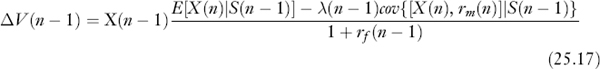
where E now refers to an expectation conditional on state S (n 1), as denoted by the vertical bars in equation (25.17). The covariance term is also calculated in this conditional manner. Note that not all the terms on the right-hand side of equation (25.17) are observable before time n.

Once we have ΔV(n − 1) calculated, we can use it in an expression just like equation (25.17) to calculate ΔV(n − 2). We can then continue to apply our single-period valuation model to each period successively so that, in general, we have at time k

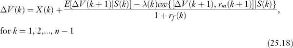
For a project with an n-period life, the technical calculation required by equation (25.18) is that of solving an n-stage stochastic dynamic programming problem. In principle,¹⁴ this approach shows how to value assets that can be traded only in imperfect secondary markets.

We shall shortly provide an example of how the approach just outlined can be put to work in solving a multi-period asset acquisition problem, but before doing so, it is instructive to compare the foregoing solution to that obtained when there is a perfect secondary market for real capital assets. A perfect secondary market fully reflects the discounted future earning power of a project at each point in time. That is, just as in the certainty case discussed in Chapter 6, a project's value at any point in time, ΔV(k), will equal its market price whenever asset markets are perfect. Note also that even if there are not perfect markets for the capital goods themselves, the same result will obtain if claims to the goods (financial instruments conveying ownership rights, such as stocks and bonds) can be sold separately in a perfect capital market. Usually, however, since the capital goods will be only a portion of the firm's assets, financial claims for the separate assets will not be available.

25.5.3 Example

Consider a project with only one operating cash flow, to be realized at time 3. First we find the project's incremental value at time 2:

The time 1 incremental value is then:

Transposing the denominator of the right-hand side of equation (25.19) to the left-hand side, taking expectations, and rearranging, we have:

Our notation now includes random variables because, while equation (25.20) provides an expression formed from the vantage point of time 2, equation (25.21) views the outcomes from the vantage point of time 1. Such variables as r_f (2), known with certainty at time 2, are known only as random variables at time 1.

Rearranging equation (25.20) into an expression for E[ΔV(2)], substituting into equation (25.21), and rearranging further, we obtain:

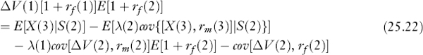
This somewhat complex-looking result has an interesting interpretation. The time 1 value of the single risky operating cash flow two periods in the future is given by the current (conditional) expectation of that flow adjusted by three risk premiums and discounted by the compound amount of the current risk-free rate and expected risk-free rate one period hence.

• By taking the expected cash flow and subtracting the first adjustment on the right-hand side of equation (25.22), effectively we obtain the certainty equivalent value viewed one period hence.
• The second adjustment accounts for the covariation risk of the intermediate value of the project one period hence, compounded to the end of the second period. This term plays the role of a reinvestment opportunity cost, accounting for the possibility that the project could be sold before the final cash flow is realized.
• The third adjustment accounts for the risk of interest rate fluctuation, since possible changes in market interest rates could affect the project's value at intermediate periods even if the other data and forecasts remain unchanged.

In a practical attempt to use this model, we might assume that the risk-free rate and market price of risk would be constant over the relevant planning horizon. This implies that the last term of equation (25.22) (i.e., the interest rate risk adjustment) is zero. We also assume the cash flow forecast is given unconditionally. Then the simplified valuation model is:

This expression can then be compared with the initial investment cost to determine whether the project is acceptable.

One interesting feature of equation (25.23) is that the reinvestment opportunity cost represented by the second right-hand term remains,¹⁵ because the opportunity cost of retaining an existing asset has to be considered in deciding whether to retain or sell it. In the general solution, the NPV of this second-period decision must be positive to continue holding the asset. Otherwise the resale value should be used instead. On the other hand, if the real capital good is fixed in the sense that it is installed at time 1 and cannot be resold at any positive price after installation, the second term of equation (25.23) is meaningless and equal to zero.¹⁶

If there were an intermediate operating cash flow X(2), it should be clear that we would add another one-period valuation expression for it to the right-hand side of equation (25.23) to obtain the appropriate expression for ΔV (1) in this case.

25.5.4 The Source of Risk

Let us rework equation (25.16) to express the value of a single uncertain cash flow X(t) at time t = 1:

How we take the next step in working backward in time and write the increment in value at time t − 2 depends on where we incorporate risk into the various arguments of equation (25.24). As Fama (1970) and Fama and MacBeth (1974) have shown, in a market where securities are priced each period according to the CAPM, there can be no relationship between risky returns realized at t − 1 and risk about the characteristics of the portfolio opportunity set to be observed at t − 1 [i.e., the point distribution of returns for period t, which in turn implies λ (t − 1)]. Should such a relationship exist, investors would have an incentive to use their portfolio decisions at time t − 2 to hedge against risk regarding portfolio opportunities available at time t − 1. These actions imply a pricing process different from the CAPM that we have been using.¹⁷

Considering the pricing model given by equation (25.24), stochastic variation in r_f (t) and λ (t) would, in general, affect the increment in the value of the firm at time t − 1, creating the type of relationship between returns realized at t − 1 and the parameters of the portfolio opportunity set at t − 1, which generally must be ruled out in multi-period applications of the CAPM. Hence, if we wish to continue to apply the CAPM, we must assume that the market parameters do not vary stochastically through time.¹⁸

Since we have ruled out risk in determining the market parameters, the only remaining source of risk about the incremental value of the firm at earlier points in time must be found with respect to the value of E[X(t)] and to cov[X(t), r_m(t)] prior to time t. If we believe that the expected value and covariance are known in all earlier periods, then we may write:

and by repeated application,

where E[r(t)] is the risk-adjusted discount rate applied to X (t) at time t. Note particularly that under the assumption that E and cov are known, the risk-adjusted discount rate is relevant only at t when the cash flow X(t) is to be realized. For the intermediate times, the risk-free rates must be applied. This appears contrary to the intuitive and widely used method of applying a risk-adjusted discount rate during all time periods.

Fama (1977) goes on to propose a rational expectations adjustment model, which allows for risk with respect to learning over time¹⁹ about the distribution of X (t). By an argument we shall not repeat here, it is shown that the only admissible risk must be isolated in the expected value of X(t) at earlier times. Under this assumption, it can further be shown that we may write:

duly noting that the expectation operator is itself time subscripted. Further, as argued above, the risk-adjusted discount rates (which are themselves derived from the covariance of the expectation adjustment variable with the market) must be known (i.e., must be non-stochastic).

Equation (25.27) looks more like what we earlier found under certainty in Chapter 6. Note, however, that in order to assume the risk-adjusted rates are non-stochastic, we have had to place heavy restrictions on the market price of risk, the risk-free rate of interest, and the reassessment risk. These restrictions are implicit in the presumption that prices in the capital market are determined each period according to the CAPM. If we further assume that these parameters are constant over time,²⁰ then the risk-adjusted discount rates will be the same in each period. This agrees more closely to the cost-of-capital approach presented in introductory textbooks in finance.

To this point, however, we have only considered a single cash flow occurring at some future time t. We now extend this to the case of finding the market value of cash flows in each of many future periods. We now rewrite equation (25.27) for a single operating cash flow, adding another subscript to the risk-adjusted discount rates to indicate that they all apply to the particular cash flow to be realized at t:

where τ runs from 1,…, t.

The total incremental value of the project then will be the sum of the incremental values of all future cash flows:

From equation (25.29) we conclude that in a capital market where prices in each period are set according to the CAPM, the discount rates E[r(t, τ)] are known but that the rates for the different periods with respect to a particular operating cash flow need not be the same and, further, that the rates for a particular period can vary across cash flows. If the firm is composed of projects of different types, we may first value individual projects as in equation (25.29) and then sum across projects to find the value of the firm. Thus, under the current assumptions, risk-adjusted discount rates can differ (1) across time for the operating cash flow of a given project to be received at a given time, (2) across the operating cash flows of a given project at any particular time, and (3) both ways as well as across the cash flows of different projects. While strictly correct under the current assumptions, equation (25.29) implies a heavy data collection burden on management.

If we write:

then we may also write the multi-period security market line as:

Again, pricing according to the CAPM implies that the values of E[r(t, τ)] and β(t, τ) are already known at time 1 but that they may vary both across the operating cash flows of different time periods t and across time τ. It may appear convenient to assume that, at least for the cash flows of projects of a given type, the values of β (t, τ) are the same for all t and τ so that the value of β is constant through time. Of course, this is just another way of saying that the required return (cost of capital) for projects with a particular cash flow risk is constant through time.

KEY POINTS

• Capital budgeting projects typically involve risk, with risk arising from different sources that depend on environmental conditions, the industry in which the firm is operating, and the type of project being considered.
• The sources of risk in capital budgeting include the risks associated with future economic, international, and market conditions, future tax rates, and future interest rates.
• In capital budgeting under risk, a firm's managers can still implement the market value criterion applied in a perfect capital market by relating that criterion to the firm's expected earnings and risk characteristics.
• The Capital Asset Pricing Model provides a theoretical framework for how risky future cash flows can be evaluated in order to assess risky projects.
• In evaluating the cash flows of risky projects, management can use a certainty equivalent approach or a risk-adjusted discount rate approach.
• In evaluating a risk project, the nature of the firm's business risk is determined by the investment projects it accepts; adopting a new project changes the firm's business risk, as reflected by the change in beta and hence in the discount rate applied to the firm's total earnings stream.
• Management should adopt new projects when their internal rate of return exceeds the market-required rate of return for projects with a given measure of risk.
• Because of the possibility of different business risks, the required rate of return on a project is not necessarily the firm's prevailing cost of capital.
• The adoption of a profitable project by management can alter a firm's overall cost of capital because the risk of the firm's earnings stream can be altered by a new investment project.
• The CAPM can be employed to develop optimal capital budgeting rules similar to those rules that management should follow in a perfect capital market.
• The rule that management should follow in assessing projects having the same business risk as the existing firm and has constant returns to scale is that such projects should be adopted provided they can be implemented at a cost low enough to permit the project to earn at least the required rate of return.
• When implementing a project that has diminishing returns to scale, management should invest up to the point where the certainty equivalent marginal internal rate of return equals the risk-free rate of interest.
• Holding output levels fixed, the CAPM can be used to relate rates of return on different projects both to each other and to the market-required rate of return.
• With fixed output levels the firm can be regarded as a portfolio of investment projects and the firm's required return is the weighted average of the returns required by the market on each of the individual projects.
• When operating incomes are risky, a project's depreciation tax shield may have to be considered risky but the depreciation tax shield will not necessarily present the same risk as the after-tax income from the project. As a result, a project's acceptability is assessed by applying different discount rates to the cash flows and the tax savings.
• A project's depreciation tax shield can be discounted at the risk-free rate, but the cash flows from operations must first be converted to their certainty equivalent value before discounting at the same risk-free rate.
• Multi-period formulations of the investment problem are useful in imperfect capital markets when the investment's cash flows occur at several moments in time.
• One way of calculating the present value of a multi-period project is to use dynamic programming to determine values sequentially. The method proceeds backward in time, one period at a time, from the horizon to the first time period. In each period's calculation, future values are added to the current value, thus providing the present value of all the project's cash flows at the first time period.
• A multi-period formulation accounts for the covariation risk of the intermediate value of the project in each of the future periods. The multi-period method in effect provides information regarding reinvestment opportunity cost, accounting for the possibility that the project could be sold before the final cash flow is realized.
• The multi-period method also takes into account the risk of interest rate fluctuation, since possible changes in market interest rates could affect the project's value at intermediate periods even if the other data and forecasts remain unchanged.
• The multi-period method provides for contingency planning, since at each period decisions to change the investment (e.g., increase, abandon) can be taken into account in the calculations, and the changes can be dependent on receiving new information or the realization of other environmental changes.

QUESTIONS

1. What are the reasons why a firm's management should not always evaluate projects with the net present value (NPV) method by direct cash flow discounting methods using a risk-free interest rate?
2. What are the three terms of the time 1 value of the single risky operating cash flow two periods in the future?
3. In the multi-period valuation model, why does the risk-adjusted discount rate need to apply to cash flow at time t, but risk-free rates are applied for the intermediate times under the assumption that the expected value and covariance of the cash flow are known?
4. The market value of a firm at time 1 is $5 million and its estimated beta is 0.4. Suppose that following the adoption of a new capital budgeting project, the required rate of return increases to 9% and the new market value increases to $5.5 million. Using the Capital Asset Pricing Model, what is the required rate of the return for the new project? Assume that the risk-free interest rate is 5% and the expected return on the market is 10%.
5. The market value of CourantRox Corporation is $20 million. There are three mutually exclusive potential projects—A, B, and C—being considered by management. Only one of the projects can be selected. All three projects require the same initial cash investment of $7 million. All three projects have only one cash flow after the project is completed one year from now. The management of CourantRox Corporation has the following information about these three projects:
   • Project A: A known single cash flow (i.e., a deterministic cash flow) of $10.5 million immediately after the completion of the project.
   • Project B: A risky cash flow (i.e., a stochastic cash flow) of $11 million and the estimated beta for this project is 0.6.
   • Project C: A risky cash flow (i.e., a stochastic cash flow) of $12 million and the estimated beta for this project is 2.1.

     The one-year risk-free interest rate (i.e., the relevant interest rate over the life of the three projects) is 5%. Based on the projections of Wall Street analysts, the expected return on the stock market over the next year is 12%.

     Given this information and assuming that the Capital Asset Pricing Model is appropriate for evaluating these three projects, which project should management prefer?

6. A group of investors is considering starting a firm. The joint distribution of the internal rate of return (IRR) for starting the firm R_j and the market portfolio return R_m is assumed to be as follows:

   

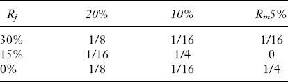
   1. What is the expected return for the market and for the firm?
   2. What is the beta for the firm?
   3. Should the investor group start assuming that the distribution above is correct and the risk-free interest rate is 5%?
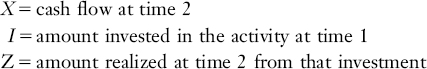
7. Assume that funds invested at time 1 produce cash flow at time 2 according to

   Z = I^½X + (1/8)log(I)X

   where

   X = the cash flow at final time

   I = amount invested in the activity at initial time

   Z = amount realized at final time from that investment

   [This is a modification of equation of (25.5) in the chapter.] Find an appropriate expression for the optimal amount of the investment in the activity at time 1.

8. The operating cash flows from a project consist of two components: (1) operating cash flow before the benefits attributable to the depreciation tax shield denoted by X and (2) the depreciation tax shield denoted by T. If the depreciation tax shield is unrelated to the outcomes of that project, using the Capital Asset Pricing Model, what is the present value of the project assuming the expected of the market return is 15% and the expected of the project E (X) is $10 million, assuming that beta is 0.3, T is $2 million, and the risk-free interest rate is 5%?
9. a. A project has cash flow at time 3 with an expected value, denoted by E[X (3)], of $5 million. What is the simplified valuation of the time 1 increment to market value, denoted by V (1) (not including investment cost), resulting from the project's adoption, assuming a constant risk-free interest rate of 5% and constant market price of risk of 0.3, the covariance of the cash flow at time 3 and market return is 4, and the covariance of the time 2 incremental value and market return is 2.

   b. What is the value of the time 1 increment to market value V (1) if there is another cash flow X (2) with an expected value of $3 million and the covariance of the cash flow at time 2 and market return is 2?

10. Assume the following about an investment project with a cost of $1,500 that is being considered by management:
    • The project will generate cash flow X (2) at time 2 that is normally distributed with mean $1,000, and standard deviation $100.
    • The project will generate cash flow X (3) at time 3 that is normally distributed with mean $1,200 and standard deviation $200.
    • The market return is normally distribution with a mean of 10% and standard deviation 0.005.
    • The correlation between X (2) and the market return is 0.8.
    • The correlation between X (3) and the market return is 0.4.

      How would management value the project if the borrowing and lending rates in the market are 8% and the project cannot be resold?

REFERENCES

Bogue, Marcus C., and Richard R. Roll. (1974). “Capital Budgeting of Risky Projects with ‘Imperfect’ Markets for Physical Capital,” Journal of Finance 29: 601–613.

Fama, Eugene F. (1970). “Multi-Period Consumption-Investment Decisions,” American Economic Review 60: 163–174.

Fama, Eugene F. (1977). “Risk-Adjusted Discount Rates and Capital Budgeting under Uncertainty,” Journal of Financial Economics 4: 3–24.

Fama, Eugene F., and James D. MacBeth. (1974). “Tests of the Multi-Period Two-Parameter Model,” Journal of Financial Economics, 1: 43–66.

Fama, Eugene F., and Merton H. Miller (1972). The Theory of Finance. New York: Holt, Rinehart, and Winston.

Long, John B., Jr. “Stock Prices, Inflation and the Term Structure of Interest Rates,” Journal of Financial Economics 1: 131–170.

Merton, Robert C. (1973). “An Intertemporal Capital Asset Pricing Model,” Econometrica 41: 867–887.