10

CONTINGENT CLAIMS AND CONTINGENT STRATEGIES

This chapter introduces the concepts of contingent claims and contingent strategies. Both are tools for analyzing and valuing the effects of risky financial decisions, and both are used extensively in the rest of the book. Indeed, we later show how contingent claims can be used to value any financial instrument, including such apparently exotic instruments as put and call options and convertible securities. We also provide further examples of how contingent strategies can be used to improve payoffs from risky decision making, as well as how they can be interpreted as ways of valuing real options.

We begin by explaining the notion of states of the world, a way of classifying risky outcomes whose value can then be represented using contingent claims. After providing examples of valuation using contingent claims, we introduce the concept of incomplete markets, and consider its importance for explaining real-world financial arrangements. We then examine some financial instruments and arrangements that can be used to trade or to manage risks. We also show how contingent claims analysis provides an alternative way to establish the Modigliani-Miller theorem about capital structure explained in Chapter 5. Finally, we discuss using contingent strategies: how decisions can differ in different states of the world, and how payoffs may be improved by making decisions that are contingent on the currently prevailing state of the world.

10.1 STATES OF THE WORLD

The idea of states of the world is useful for thinking about convenient ways to model risky payoffs. In a two-time-point model, states of the world are defined as those future events that matter to the decision problem being considered. These states of the world are defined by the decision maker to be mutually exclusive and collectively exhaustive. Using an example given by Savage (1951), if one is about to break a ninth egg into a bowl already containing eight other eggs, the relevant states of the world could be whether or not the ninth egg is rotten and would hence spoil the others. (Here we presume the rottenness of an egg is not discernible until the egg has been broken and fallen into the bowl.)

In a second example more closely related to finance, an investor might be concerned with the future price of a share of stock, and this price might in turn depend on economic conditions. Suppose the investor defines (1) “states” to represent economic conditions and (2) “future prices” to be the following list of possible stock prices that may be realized at the time a given state is actually realized:

State	Future Prices
1	$10
2	$ 8
3	$ 6

For example, state 1 might mean that the industry in which the firm operates faces buoyant market conditions; state 2, conditions that are neither good nor bad; and state 3, conditions that are depressed. In each state, the effect is registered on the stock price. We shall usually associate probabilities with the states; for example, p_i might represent the probability that state i will actually occur; that is, i = 1, 2, 3. Because the states are mutually exclusive, only one can actually occur; because they are collectively exhaustive, one of the three must occur. Hence, ∑p_i = 1.¹

10.2 CONTINGENT CLAIMS AND THEIR VALUE

A unit contingent claim is a security that will pay an amount of $1 if a certain state of the world is actually realized, but nothing otherwise. A claim that pays $1 if state i is realized is frequently called a unit claim on state i. A unit contingent claim is also referred to as a primary security or Arrow-Debreu security.² Accordingly, the future stock price described in Section 10.1 may be regarded as equivalent to a package containing all of the following:

Ten unit claims on state 1

Eight unit claims on state 2

Six unit claims on state 3

The idea of a contingent claim is thus useful for expressing, in terms of fundamental units, exactly what a given security's payoff may be in different possible states of the world.

It may take a little imagination to come up with real-world examples of claims, and those real-world examples are not numerous.³ But packages of unit claims represent perfect substitutes for the more ordinary types of securities such as stocks or bonds, and we shall frequently find it useful to employ claims to help understand price relations between securities. For example, if we assume a perfectly competitive financial market along with a description of future events in terms of states of the world, certain price relationships between securities and contingent claims must be obtained. This means in turn that certain predictable relationships between securities prices must also be obtained, as introduced next and as examined further in Chapter 16.

To see these relationships, suppose that we can describe the world using two states and that two stocks are available, stock A and stock B. We assume the stocks’ future prices have the following distributions:

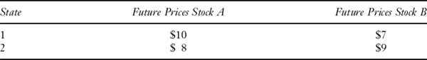
Let A(1) = $6 denote the time 1 price of stock A, B(1) = $5 the time 1 price of stock B, and suppose these prices admit no arbitrage opportunities. Now, if we let C₁ and C₂ represent the time 1 prices of unit claims on states 1 and 2, we can use the foregoing information about stock prices and payoffs to find the time 1 prices C₁ and C₂. Purchasing stock A for $6 is equivalent to buying a package of 10 unit claims on state 1 and 8 unit claims on state 2, while buying stock B for $5 is equivalent to buying a package of 7 unit claims on state 1 and 9 unit claims on state 2. Since the unit claims comprising the two stocks are perfect substitutes, they must sell for the same prices in a perfect market. Hence, we can write:

which can be solved to obtain:

We can use the same reasoning to find the risk-free rate of return that must be obtained in this market. Since a risk-free instrument is one that offers the same payoff irrespective of which state of the world obtains, we wish to find a combination of the two stocks that gives the same time 2 payoff, here denoted k, in either state of the world. That is, the following equation must be solved for α:

We can write the payoff k as equal to either of the following payoffs:

10α + 7(1 − α) = 8α + 9(1 − α)

which implies that:

2α = 2(1 − α)

so that . The riskless payoff is then , and this can be obtained for a price equal to , since a portfolio composed of equal proportions of the two stocks creates the riskless investment. Accordingly, the risk-free rate of return is:

Of course, this is not necessarily a realistic number for a risk-free rate of interest.⁴ However, our purpose here is to develop illustrative calculations to display relations between contingent claims, and for this purpose particular sizes of numbers are not really important.

Another way of making a riskless investment is to buy one of each available unit claim, that is, one claim on state 1 and one claim on state 2. Such a portfolio gives a certain payoff of $1 for an investment cost:

The rate of return on this investment is then:

just as before.

10.3 INVESTOR'S UTILITY MAXIMIZATION IN CONTINGENT CLAIMS MARKETS

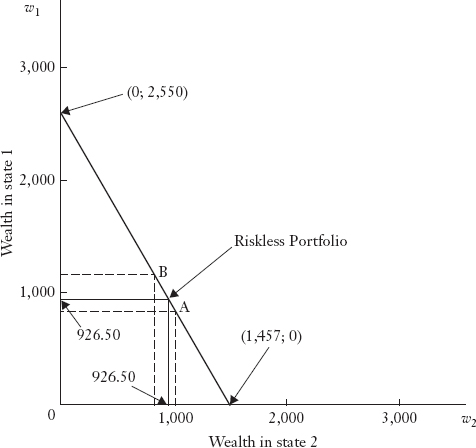
In this section we describe how an investor can solve the utility maximization problem when facing risk in a market for contingent claims. For our illustration, we shall continue with stocks A and B from the previous section. Further, we shall assume the investor's initial wealth to be $600. This scenario is summarized in Table 10.1. We let w₁ represent wealth if state 1 occurs and w₂ represent wealth if state 2 occurs. We can plot these data in (w₁, w₂) space as shown in Figure 10.1. Note that the previously determined riskless position of dividing the purchases to obtain an equal number of each security (54.5 of each) generates a riskless terminal wealth position of w₁ = w₂ = $926.50.

TABLE 10.1 SUMMARY OF TERMINAL WEALTH IN TWO STATES

FIGURE 10.1 MARKET OPPORTUNITY LINE SHOWING IMPLIED PRICES OF UNIT CLAIMS

We can also use another way to calculate the value of the claims’ combinations at time 1. We can write the equation of the straight line in Figure 10.1 as:

w₂ = a − bw₁

so that for the time 1 price of stock A we have:

$800 = a − $1,000b

while for the time 1 price of stock B we have:

$1,080 = a − $840b

Solving these two simultaneous equations, we find b = 1.75 and a = $2,550. Thus, when w₁ = 0, w₂ = $2,550, while when w₂ = 0, w₁ = $1,457, which are the two intercepts of the line on their respective axes in Figure 10.1.

Now if w₂ = 0, we have the case of a claim (primary security) on state 1. (The security pays $1,457 in state 1 and nothing otherwise.) The price of this claim can be calculated by dividing initial wealth by the maximum wealth obtained if state 1 occurs, or $600/$1,457 = 0.41. Similarly, the price of primary security 2 is $600/$2,550 = 0.24(= 4/17), the same values as obtained previously.

Note that in Figure 10.1 the investor's time 1 position is some point on the line from A to B. How could the investor obtain a terminal wealth position lying beyond these points? The investor could engage in short sales, that is, selling shares not currently owned, for delivery when the unknown future state of the world is revealed. In this transaction the investor obtains cash from the time 0 sale of one security and uses it to buy the other. In so doing, the investor promises later to buy the security sold short at whatever price will be prevailing and deliver it. Note that there is a potential for large gains or losses in such transactions. Here the initial wealth will be used as a constraint and we shall require that at worst the investor will have zero terminal wealth if he guesses incorrectly. That is, no net borrowing is permitted at the end of the period so that the investor cannot go beyond the intercepts in Figure 10.1.

To illustrate, consider point w₁ = $1,457, w₂ = 0. Let n_A be the number of shares of stock A and n_B the number of shares of stock B purchased. If state 1 occurs, the terminal wealth will be:

10n_A + 7n_B = $1,457

while if state 2 occurs, we must have:

8n_A + 9n_B = 0

Solving these equations simultaneously, we find n_B = −343. If the investor sells short 343 shares of stock B at the current price of $5, he will receive $1,715. Combining this with the initial wealth of $600 gives $2,315, so this investor may buy $2,315/$6 = 386 n_A at $6 per share. If state 1 eventuates, the investor will receive $3,860 ($10 times 386 shares) but now must pay $2,401 ($7 times 343 shares) for stock B shares to cover the short position. The net terminal wealth is $3,860 − $2,401 = $1,459 (difference due to rounding), as required. In state 2, the terminal wealth will be equal to $3,088 (386 shares times $8 per share) reduced by the cost to repurchase stock B to cover the short position, 343 shares at $9 per share or $3,087. Therefore, the net terminal wealth is equal to zero (the calculations show it is $1 but that is due to rounding).

Note that none of the points we have considered will necessarily be a utility-maximizing point. To determine this point, it is necessary to know the investor's utility function in (w₁, w₂) space. Given a utility function, the investor's utility-maximizing position is the familiar one discussed in Chapter 2. The optimal portfolio for the investor satisfies the tangency condition that the slope of the wealth constraint (the ratio of the prices of the unit claims) equals the slope of the indifference curve (marginal rate of substitution of state 1 consumption for state 2 consumption).

The immediate purpose of the foregoing demonstration is to show that every security can be viewed as a bundle of unit claims and thus represents a combination of positions regarding future states of the world. Moreover, in these circumstances an investor can attain any point along the market opportunity line. If, on the other hand, there are fewer securities than the number of distinct states, the individual's optimal consumption choices may not be attainable. The significance of this will be explored in the next section.

The second purpose, although it is not yet clearly revealed, is to demonstrate that contingent claim analysis provides a powerful method for valuing complex financial instruments and financial arrangements, as will be shown in Chapters 17 through 19.

10.4 INCOMPLETE MARKETS FOR CONTINGENT CLAIMS

A market is said to be a complete market when economic agents can structure any set of future state payoffs by investing in a portfolio of unit continent claims (i.e., primary securities). A financial market is said to be incomplete if the number of (linearly) independent securities traded in it is smaller than the number of distinct states of the world. Clearly, market incompleteness depends on how states of the world are defined. However, since the number of states of the world used to describe a typical financial market is likely to be large,⁵ the possibility that real-world financial markets will be incomplete is a very real one.

The importance of market incompleteness is best introduced by an example. Let us consider an economy with three possible states of the world and suppose only two securities (taking the form of unit claims for ease of exposition) are traded in it. Table 10.2 describes the securities in terms of their time 1 payoffs for each state of the world. It is apparent from the table that weighted averages of the two unit claims can be used to create packages with time 1 distributions of values ranging between zero and unity, the actual outcome depending on whether state 1 or state 2 is realized. However, by using just the existing two unit claims, an investor cannot create an income claim of other than zero in state 3. Moreover, no investor can arrange a risk-free investment in this example, because it is not possible to guarantee the same return in every state of the world by using the available securities.

TABLE 10.2 MARKET VALUES OF TWO SECURITIES AT TIME 1

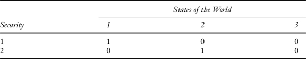
The situation is quite different if a third unit claim worth $1 in state 3 and zero in the other states becomes available. Now the number of claims equals the number of distinct states, and a risk-free investment can be arranged.

We are now ready to discuss some practical implications of market incompleteness. It is obvious from the foregoing example that investor choice is restricted in incomplete markets. Moreover if investor choices are restricted, the investors will never be better off, and are likely to be worse off, than would be the case if markets were complete (i.e., if the restrictions were removed). In such situations, it is to be expected that if ways of completing the market can be found, those possibilities are likely to be utilized. That is, in the context of incomplete financial markets the appearance of new instruments might be regarded as attempts to provide investors with financial opportunities not otherwise available. The appearance of derivatives (options, futures, and swaps) can be regarded as examples of such attempts. Mossin (1977) argues that the preference existing firms show for organizing new activities as separate corporations may be another indication of attempts to deal with market incompleteness.

We shall have more to say about recently created financial instruments, their relations to incomplete markets, and their pricing in later chapters. For the present we wish next to indicate some of the ways in which real-world financial instruments and arrangements can be interpreted as contingent claims.

10.5 MODIGLIANI-MILLER REVISITED

Let's revisit the Modigliani-Miller theorem of Chapter 5 using contingent claim analysis. Our purpose is to provide a different illustration of how the securities a firm issues can be regarded as representing only a division of the firm's operating earnings.

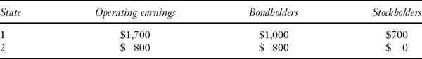
Let p(s) be the price at time 1 of receiving $1 at time 2 if state s is realized. That is, p(s) is the time 1 price of a unit claim that pays $1 at time 2, if state s then occurs. Now suppose management raises funds by issuing a bond that promises to pay $500 (which includes interest and face value) at time 2. Continuing to assume that there are only two possible states that can be realized at time 2, and that the firm can generate operating earnings in each state as shown below, the bondholder and stockholder claims are also as shown:

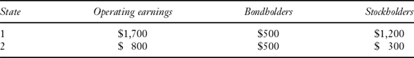
Using the prices of the contingent claims, the value of the bond at time 1, denoted by B(1), is:

B(1)= $500 p(1) + $500 p(2)

In other words, to rule out the possibility of arbitrage, the value of the bonds must be just equal to the value of a package of contingent claims constituting a perfect substitute for the bonds. Similarly the time 1 value of equity, denoted by S(1), is:

S(1) = $1,200 p(1) + $300 p(2)

Finally, the value of both securities (a value that also represents the market value of the firm), denoted by V(1), is:

V(1)= $1,700 p(1) + $800 p(2)

Notice that the market value of the firm is just the sum of the market values of the two securities, as it must be under the Modigliani-Miller assumptions.

The calculation shows that payoffs on the firm's securities, and payoffs on the firm itself, can be regarded as packages of contingent claims. Any different set of packages will have the same combined value, so long as the payoffs add up to the firm's entire earnings. To see this, consider a second case in which bonds promising to pay $1,000 at time 2 are issued. The distribution of the claims is then:

Since these bonds will be partially defaulted in state 2 because the payoff is less than the required bond payment, the time 1 value of the bonds is:

B(1) = $1,000 p(1) + $800 p(2)

and the time 2 value of equity is:

S(1) = $700 p(1) + $0 p(2)

But this still means the time 1 value of both securities together is as given earlier for V(1):

V(1) = $1,700 p(1) + $800 p(2)

The importance of this discussion is threefold. First, it uses a different method to confirm the irrelevance of capital structure based on the assumptions made by Modigliani and Miller as established in Chapter 5. Second, it demonstrates that bonds and equity merely represent different ways of packaging the fundamental units (contingent claims) that can be regarded as representing the firm's earnings. Under the assumptions of the Modigliani-Miller analysis, different ways of packaging fundamental units have no effect on the total numbers of each kind of fundamental unit represented by the firm's earnings. Third, the discussion here shows how easy it is to apply contingent claim analysis to valuing different securities. In essence the demonstration shows that financial theory values different kinds of securities, no matter how complex, in exactly the same way. In each case the basis of a security's value is the package of fundamental units it represents.

10.6 FINANCIAL INSTRUMENTS AS CONTINGENT CLAIMS

Most financial instruments can be bought or sold, but not all of them are actively traded in financial markets. For example, a common form of contingent claim (and one that is close in concept to a unit claim) is a lottery ticket. In its simplest form this claim results in its holder winning either a positive prize or zero. Accordingly, this lottery ticket represents a claim that can be valued using two states of the world.⁶ But lottery tickets, once issued, are rarely traded again. The same is true of such other contingent claims as the tickets obtained when betting on horse races or similar contests.

An insurance policy is a contingent claim that comes closer to our usual notions of a financial instrument, but traditional forms of insurance policies are rarely traded in the financial markets. On the other hand, put or call options, representing contingent claims for selling or buying securities or financial indices at prespecified prices (options will be discussed extensively in Chapters 18 and 19), trade actively on such organized exchanges. Rights and warrants are other examples of contingent claims in that they permit, but do not require, the holder to buy securities on prespecified terms.

There are also securities that have embedded derivatives in them, derivatives that are not traded separately from the instrument itself. For example, a callable bond is a bond that grants the issuer the right to redeem the bond at some time in the future and at a specified price. That is, a callable bond can be viewed as a straight bond with an embedded call option granted to the issuer. A putable bond is a bond that grants the investor the right to sell (i.e., put) the bond to the issuer in the future at a specified price. Hence, the bond structure can be viewed as a straight bond with an embedded put option. Convertible securities, which include convertible bonds or convertible preferred stocks, represent contingent claims in that they typically allow the owner to exchange the original issue for other securities, usually common stock, and they are callable. Some convertible securities even include an embedded put option.

A number of other commonplace financial arrangements, again not usually traded in the marketplace, also can be regarded as contingent claims. As suggested by Brennan (1979), these include such possibilities as a firm's tax liability, which is dependent on the size of its taxable income.⁷ In this case the relevant states of the world are economic conditions that affect reported income. Tax shields on depreciation or leasing expense will be valuable only if there is sufficient operating income. Costs that will be paid only in the event of a firm facing technical insolvency represent another kind of contingent claim on the firm. Finally, the opportunities a firm may have to make future investments (investments with varying degrees of profitability) or to purchase physical assets when a lease expires also represent contingent claims owned by the firm.

The realization of many of these opportunities is often dependent on the firm's using contingent strategies (taking different decisions in different states of the world), a matter to which we next turn.

10.7 CONTINGENT STRATEGIES

Just as investor satisfaction can increase if more kinds of contingent claims become available, a firm can improve its earnings distribution⁸ by using a contingent strategy. To recognize the possibility of taking contingencies into account in decision making, we say a decision maker uses contingent planning when instead of merely saying “I will do X,” the person announces “I will do X₁ if state 1 is realized, X₂ if state 2 is realized,” and so on.⁹ The details of contingency planning are referred to as formulating a contingent strategy.

Just as an insufficient number of securities can restrict investor satisfaction in an incomplete market, an absence of contingent planning can lead to less desirable payoff distributions than might otherwise be available. To establish the connection between contingent claims and contingent strategies in greater detail, we first discuss the context in which contingent strategies arise and then provide an example showing how contingent planning can effect improvements over noncontingent decision making.

Consider a firm planning to select a location and build a factory now in the hopes of later expanding its facilities if its products can successfully be marketed. The initial location decision cannot easily be reversed and will affect future payoffs earned by the firm. For example, the kinds of expansion activities that may later take place will very likely depend on the initial location and what may be learned about it in the future. It might be that at one location a complete product would be produced, while at another location components would be produced for assembly still elsewhere. In any event, once a given location has been selected, the type of expansion plan selected will depend on the initial location choice. Furthermore, the details of that type of expansion plan may change as time passes, because more is likely to become known about local conditions after the initial location decision has been made. Accordingly, management has a choice: select now the location that offers the highest criterion function value if the future turns out as anticipated, or alternatively, select the location most suitable for taking a variety of possible decisions if the future turns out to differ from the most likely scenario presently anticipated. The latter is a form of contingent planning.

TABLE 10.3 DECISION SEQUENCES AND THEIR PAYOFFS

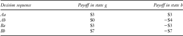
To develop the details of computations related to contingent planning, we present a numerical example. In doing so, we assume the particular decision problem discussed can be considered separately from others faced by the firm. Also, for simplicity we assume that the firm wishes to maximize the expected value of the payoffs involved.¹⁰ Esoteric Electronics is a manufacturer of components used in both industrial applications and in space exploration. At the present time, the company is planning its production for the next two quarterly periods. It has to decide whether to produce either a or b components in each quarter, since it cannot produce both components simultaneously. Steady production of either one component or the other for both quarters eliminates setup charges. On the other hand, revenues from continued production of b will be affected by the success or failure of a space exploration mission, the results of which will become known before the end of the first quarter but after the time for making the first quarter's production decision has passed. The revenue from a, a non-space-industry-utilized component, is independent of the mission's outcome.

The foregoing considerations are captured in Table 10.3, where production plan payoffs are shown to depend on the state of the world (i.e., the mission outcome). A successful mission outcome is denoted by g and an unsuccessful outcome by h. The sequences of events are also displayed in decision tree form in Figure 10.2.

Now suppose that the best presently available estimate of the probability of a successful mission (state g) is 0.65. Management might then make the calculations shown in Table 10.4 and state that they should elect to produce a in both quarters since that gives the highest expected payoff. However, the kind of thinking used to select the strategy of producing a in both quarters proceeds along lines like the following. Long production runs are better because they eliminate setup costs. At the same time, mission success is more likely than failure, so on an expected value basis it pays to produce a in both quarters. At this point, the reader should consider how noncontingent strategies would be displayed on the tree of Figure 10.2.

The problem with noncontingent strategies in the assumed circumstances is that the actual mission outcome will be known before the second-quarter production must be determined. Although it is true that setup costs will have to be incurred a second time if switches in production are made after the first quarter, these increased costs might in some circumstances be offset by the higher payoffs realized from producing whichever product is appropriate once the mission outcome is known. Hence, it can be important to select plans that allow for this possibility of revision, especially if the most likely outcome does not occur.

FIGURE 10.2 ILLUSTRATION OF A CONTINGENT STRATEGY

TABLE 10.4 NONCONTINGENT STRATEGIES AND EXPECTED PAYOFFS

Noncontingent Strategy	Expected Payoff
a(ga, ha)	$3(0.65) + $3(0.35) = $3.00
a (gb, hb)	$0(0.65) + $4(0.35) = $1.40
b (ga, ha)	$3(0.65) + $3(0.35) = $0.90
b (gb, hb)	$7(0.65) + $7(0.35) = $2.10

Note: The notation c(gd, hd) means that production of c is planned for the first quarter, followed by production of d in the second quarter regardless of whether the mission succeeds or fails.

TABLE 10.5 CONTINGENT STRATEGIES AND EXPECTED PAYOFFS

Contingent Strategy	Expected Payoff
a (ga, hb)	$3(0.65) + $4(0.35) = $0.55
a (gb, ha)	$0(0.65) + $3(0.35) = $1.05
b (ga, hb)	$3(0.65) + $7(0.35) = $0.50
b (gb, ha)	$7(0.65) + $3(0.35) = $3.50

To see how this type of reasoning may be implemented, we now consider contingent strategies. These kinds of strategies may be denoted by c (gd, he), which means that production of c is planned for the first quarter, followed by production of d in the second quarter if the mission succeeds or by e if the mission fails. Notice that a contingent strategy of the type c (gd, hd) is really degenerate in the sense that it does not differ from a strategy in the noncontingent category already considered. The nondegenerate contingent strategies and their payoffs are given in Table 10.5; the complete contingent solution method considers the strategies in both Tables 10.4 and 10.5. One can use Figure 10.2 to see how a contingent strategy differs from a non-contingent strategy by imposing fewer constraints on the decision maker's choices.

From Table 10.5, we see that the optimal strategy is b (gb, ha). In other words, management begins by producing b and continues with b if the mission is successful but switches to a if the mission is unsuccessful. Note this strategy has a higher expected value than the noncontingent strategy that management initially considered. What we have shown, then, is that incorporating flexibility into the firm's decision making encompasses a wider range of possibilities, and the extra flexibility gained never does any harm (except for the costs of making extra computations). More often than not, the procedure may yield real benefits, as in the example just studied.

In other situations, the increased payoffs to contingent planning may only be available at increased cost. The problem then is to decide whether the expected increased benefits outweigh the increased costs. We shall discuss examples of financial decisions involving these issues at several points in the succeeding development. We shall see that contingent planning provides ways to redistribute both risks and information about risks. In particular, we shall discuss management's use of information about future conditions in relation to making contingent capital expenditure decisions in Chapter 26. We shall also discuss management's provision of information to investors in relation to making contingent financing decisions (e.g., issuing convertible bonds) in Part VII of this book.

KEY POINTS

• Contingent claims analysis and contingent strategies are tools for dealing with risk in financial decision making.
• Contingent claims analysis uses the notion of states of the world in assessing future risky payoffs.
• A unit contingent claim (also known as a primary security or Arrow-Debreu security) is a security that has a payoff of $1 if a certain state of the world is actually realized, but nothing in all other states.
• A contingent claim that pays off $1 if state i is realized is also referred to as a unit claim on state i.
• Although few unit contingent claims exist in reality, claims represent a useful tool to employ in valuing securities and in understanding relations among securities prices.
• An investor facing risk in a market for contingent claims may formulate her decision problem as one of utility maximization.
• Every security can be viewed as representing a bundle of unit claims and thereby further represents a combination of positions (long and short) regarding future states of the world.
• Contingent claims analysis can be used to show how an investor can affect his terminal wealth position by engaging in short sales (i.e., selling shares not currently owned, for delivery when the unknown future state of the world is revealed). The outcomes in this case are riskier than they would be in the absence of short selling.
• If the number of (linearly) independent securities traded is smaller than the number of distinct states of the world, the financial market is said to be incomplete.
• Because the number of states of the world necessary to describe a well-functioning financial market is likely to be large, the possibility that real-world financial markets will be incomplete is a very real one.
• Although many financial instruments representing contingent claims can be bought or sold, not all financial instruments or arrangements are actively traded in financial markets.
• Contingent strategies can be used by a firm's management to recognize the possibility of taking contingencies into account in financial decision making. Contingent strategies can improve the payoffs obtained from financial decision making.

QUESTIONS

1. What is the purpose of understanding:
   1. contingent claims?
   2. contingent strategies?
2. How is the concept of “states of the world” useful in making decisions under risk? Under uncertainty?
3. What is meant by a unit contingent claim and why is this concept useful in financial economics?
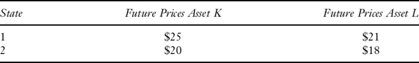
4. Suppose that we can describe the world using two states and that two assets are available, asset K and asset L. We assume the assets’ future prices have the following distributions:

   

   Let K(1) = $20 denote the time 1 price of asset K and L(1) = $19 the time 1 price of asset L.

   1. Assuming no arbitrage opportunities, what are the values of the unit claims at time 1?
   2. What is the risk-free rate of return that must obtain in this market?
5. Suppose that we can describe the world using two states. The time 1 prices for contingent unit claims on states 1 and 2 in this market are $0.3 and $0.5, respectively. An investor's utility function in (w1, w2) space is U w1, w(2) = w1 × w2, where U represents the utility level. In addition, the initial wealth of the investor is $420. What is the maximum utility portfolio for this investor?
6. What is meant by a short sale?
7. What is meant by an incomplete financial market?
8. Suppose that the world can be described using two states and two stocks Y and Z are available. We assume the stocks’ future prices have the following distributions:

   

   The initial prices for the stocks are: Y(1) = $13, Z(1) = $10. Our utility function in (w1, w2) space is U w1, w(2) = w1 × w2, where U represents the utility level. Now we have an initial endowment of $420. How many shares and what positions of Y and Z should we choose to build our portfolio so that we actually maximize our utility function? (Assume fractional shares are permitted.)

9. What are several types of bonds that have embedded options can be viewed as contingents claims?
10. Why can a firm's tax liability be viewed as a contingent claim?
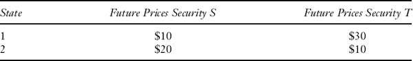
11. Henry Morton has an initial wealth endowment of $1,200. He considers the future to be risky but completely characterized by only two possible states. Henry has the opportunity to invest in two securities S and T for which the initial prices are S(1) = $10 and T(1) = $12. The payoffs to these securities are:

    

    1. If Henry buys only security S, how many units can he purchase?
    2. If Henry buys only security T, how many units can he purchase?
    3. What will be his final wealth in both cases and in each state?
    4. Suppose now Henry can issue as well as purchase securities. However, he must be able to meet all claims under the occurrence of either state (terminal wealth can be zero, but he cannot renege on any promises). Now how many units maximum of S could Henry sell to buy T, and conversely, how many units maximum of T could he sell to buy S?
    5. What now would be Henry's terminal wealth in both cases and in each state?
12. Two securities have the following payoffs:

    

    The current prices are G(1) = $8 and H(1) = $9. Both future states are equally likely. Your initial endowment (current wealth) is $720.

    1. If you wanted to purchase a completely risk-free portfolio, how many units of G and H would you buy (fractional units are permitted)?
    2. What will be the implied risk-free return?
13. Suppose there is a stock S in the market. The terminal price of S can be $40, $42, or $45. Therefore, we can describe the world in three states. There also exists a security has the payoff as follows:
    • When the terminal stock price S_T is greater than $41, it pays S_T − $41.
    • When the terminal stock price S_T is equal to or less than $41, it pays 0.

      Show that this security is a contingent claim.

REFERENCES

Arrow, Kenneth J. (1964). “The Role of Securities in the Optimal Allocation of Risk-Bearing,” Review of Economic Studies 31: 91–96.

Brennan, Michael J. (1979). “The Pricing of Contingent Claims in Discrete Time Models,” Journal of Finance 34: 55–68.

Debreu, Gerard. (1959). The Theory of Value. New York: John Wiley & Sons.

Fabozzi, Frank J., and Uzi Yaari. (1983). “Valuation of Safe Harbor Tax Benefit Transfer Leases,” Journal of Finance 37: 595–605.

Mossin, Jan (1977). The Economic Efficiency of Financial Markets. Lexington, MA: Heath.

Savage, Leonard J. (1951). The Foundations of Statistics. New York: John Wiley & Sons.