2

CONSUMER FINANCIAL DECISIONS

Consumer behavior plays a key role in determining what and how much is produced in a developed economy. For this reason, a convenient starting point in microeconomic theory is to understand the basic principles of how consumers make consumption and investment decisions. In arranging their expenditure and finance planning, consumers both spend and invest in the financial obligations of firms and governments. Firms and governments are thus borrowing from consumers who decide both how much to consume at a given time and how much to lend or invest (through the purchase of financial assets) for financing future consumption. Ultimately, the price of investment funds is determined by the interaction of lender preferences and borrower needs. Thus, consumer behavior with respect to financial decisions is critical to understanding financial economic theory.

In this chapter, we describe the basic features of consumers' financial decisions. As we do throughout this book and as explained in Chapter 1, we begin by considering the decisions made by consumers in a certainty world with a perfect capital market.¹

2.1 THE CONSUMPTION-INVESTMENT PROBLEM

In a typical developed economy, consumers' purchases determine the outcome of more than two-thirds of the output produced. Indeed, since consumer decisions are the foremost means by which goods and services are distributed in any developed economy, it is important to understand consumer behavior. To do so, we employ what is termed the theory of consumer choice. The theory of consumer choice examines the trade-offs consumers must make, because their income is limited and choices of consumption goods and services are numerous. That is, consumers must consider what they can afford and what they would like to consume. The former consideration is expressed mathematically by a budget constraint and the latter by a function that expresses their preferences.

In order to emphasize the essential features of a consumer's financial decisions, the theory of consumer choice employs a number of simplifying assumptions.² The setting we first examine has these features:

1. Every consumer lives in a world of certainty; that is, all decision-relevant information is known exactly to the consumer, now and for all future time.
2. Only two points in time are of importance, the present time and a later time that accounts for effects that may persist into many future periods. (We subsequently show how this two-period orientation satisfactorily represents financial decision problems involving many time periods.)
3. There are many transactors in the capital market, and no single transactor is large enough to affect prices or interest rates. (Sometimes, but not always, we make similar assumptions about markets for other inputs and outputs such as capital equipment.)
4. Every market participant has the same (certain) information about market prices and the relevant terms of any transaction.
5. Transactions in the capital market can be made without payment of charges other than the ruling market rate of interest.

The last three conditions together describe what is called a perfect capital market. An important consequence of a perfect capital market under circumstances of certainty is that every financial instrument is the same as every other in terms of its credit risk and the rate of interest it yields when that rate is computed on the instrument's market price. In a world of certainty, no money is lent or invested unless it is known that the borrower will repay, so credit risk does not exist at all. No user of funds need pay a higher rate of interest than any other because there are many lenders and the borrower knows the rates they all charge. Hence, there is no reason to borrow at rates in excess of the market interest rate. Also, no lender will provide credit at interest rates lower than the market rate because the market rate can always be obtained on alternative transactions.

A further implication of the foregoing is that any profile of cash receipts (or disbursements) having a given present value leaves its owner in the same wealth position as does any other profile with the same present value. That is, if market interest rates are 10% per time period, $1 available now is exactly equivalent to $1.10 available one period later, because at the same point in time either cash flow profile has the same value in the capital market. This means that in the world just described, financial decisions are easy to make, and the principles on which they are based are easy to discern. Because everyone borrows or lends at the same market interest rate (a rate that may differ from one time period to the next), financial transactions can be reduced to a single measure, that of their present value.

2.1.1 Describing Individuals’ Preferences

To explain why consumers decide to borrow or lend at different points in time, we describe both their preferences and their opportunities to reach preferred positions. Individuals' preferences can be described in terms of their attitudes toward bundles of consumption goods available at different points in time. In our context, the satisfaction provided by consuming various goods is summarized by their market value, which we refer to as a consumption standard.³ Hence, we wish to represent, in a convenient way, a consumer's preferences for money expenditures at different points in time.

Preferences can be represented conveniently, using what is called a utility function, if a consumer is able to make consistent statements about what is preferred. The technical meaning of making such statements is as follows:

1. The consumer can compare one pair of consumption standards (C₁, C₂) with another, say (), and state which, if either, is preferred.
2. The consumer can make the comparisons transitively; that is, if one consumption standard is preferred to a second, and if the second is in turn preferred to a third, then the first is also preferred to the third.

   As long as the consumer's preferences satisfy the two foregoing assumptions, attitudes toward different consumption standards can be represented by a numerical utility function that assigns a larger number to the preferred alternative, if either, of a given pair. Such a utility function also assigns equal numbers to equally preferred alternatives. Thus, a consumer who tries to attain the most preferred position available to him can be represented as trying to maximize utility.

   The form of the utility function can be illustrated as in Figure 2.1, using contour lines called indifference curves. The indifference curves represent loci of points at equal height on a utility surface defined above a plane on which time 1 and time 2 consumption standards are measured. Any point on any indifference curve represents a combination of time 1 and time 2 consumption expenditures that is as satisfactory as any other point on the same curve, as reflected by the fact that each indifference curve is a set of points for all of which the utility function attains the same value. To be sure the indifference curves will have the shape shown in Figure 2.1, we must also assume that:

3. The higher the consumption expenditure, the greater the consumer satisfaction.

   This means that increasing satisfaction is represented in the diagram by movements in north, east, or northeast directions. Finally, we assume that:

4. Any average over two equally satisfactory different consumption combinations yields a higher level of satisfaction than either of the combinations comprising the average.

FIGURE 2.1 INDIFFERENCE CURVES FOR PERIOD 1 AND PERIOD 2 CONSUMPTION STANDARDS

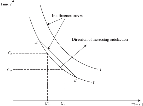
The purpose of this assumption is to render the indifference curves strictly convex. Strict convexity means that the straight line between points like A and B in Figure 2.1, indicating averages over consumption standards represented by points A and B, lies inside indifference curve I and hence actually touches curves higher than I. This assumption is used to remove any ambiguity about which set of consumption standards a consumer actually will select when the possible choices are limited.

The slope of an indifference curve at any point is called the marginal rate of substitution between present and future consumption. This rate indicates the consumer's preference for trading off consumption at the present time against consumption in the future. It will be noted by virtue of our last two assumptions that the marginal rate of substitution for consumption in a given period diminishes as that period's consumption increases. Hence, the larger is present consumption, the lower becomes the consumer's preference for additional present, rather than future, consumption. For example, as time 1 consumption increases, the indifference curves in Figure 2.1 become more nearly horizontal. This means that the higher the level of consumption in time 1, the more consumption must increase in time 1 to compensate (in the sense of leaving the consumer on the same indifference curve) for a given decrease in time 2 consumption.

2.1.2 Opportunities for Financing Consumption Expenditures

Consumers’ choices are subject to the limitations of what they can afford. The resources individual consumers can expend on consumption are assets already available and incomes that will be received. The value of available assets at a given time t is referred to as wealth at time t, w_t, and consists of the market value of stocks of real durable goods and financial assets carried over from previous periods. Income consists of wages, salaries, or other payments received at time t and will be denoted as y_t. Individuals may purchase either durable or nondurable goods, where by a durable good we mean one that lasts longer than a single time period. Nondurables have a one-period life because they are merely purchased and consumed. For the time being we assume that any durable good a consumer might wish to buy can be rented on a period-by-period basis.⁴ This means that any assets consumers hold from one period to the next will take the form of financial instruments.

Since we are presently considering a certainty world, future income is known exactly at any time. But the problem with future income (even if it is known with certainty) is that it cannot be used to finance current consumption unless the individual can somehow borrow against it. Hence, we suppose there are arrangements to permit this. These arrangements are, of course, dependent upon the ability to transact in the capital market.

As already noted, in the present analysis the capital market is assumed to be perfect. In such a market only a single equilibrium price for credit can prevail. Denote this price by p, where p is the time 1 price for delivery of $1 at time 2 (i.e., one time period later). While p indicates that there is a price for money borrowed or lent, it is usually more convenient to express this price as an interest rate. Note first that if p is the time 1 price of $1 to be delivered at time 2, we can say alternatively that $1 is the time 1 price of a sum 1/p to be delivered at time 2. The sum initially borrowed or lent increases if individuals prefer to spend money now rather than later, as will usually be the case. Assuming this to be so, p will be less than 1 and 1/p greater than 1. Then we can rewrite:

That is, we define (1 − p)/p as r, where r is the rate of interest between times 1 and 2. Just as there is only one equilibrium value of p in a perfect market, there will be only one interest rate r. We may also rewrite equation (2.1) to obtain:

showing that the price p represents the value of $1 discounted at interest rate r.

Considering now the question of the opportunities facing an individual consumer in such a world, suppose an individual has an income stream, fixed and unalterable, of y₁ and y₂ to be received at times 1 and 2, respectively, as shown in Figure 2.2. (If the individual has any financial assets, their market value can be assumed to be included in the magnitude y₁.) We next wish to determine the present value of this income combination. It is the sum of time 1 income y₁ plus the present value of income y₂; that is, y₁ + y₂/(1 + r). This sum represents wealth at time 1, and is denoted by w₁.

FIGURE 2.2 INDIVIDUAL'S WEALTH CONSTRAINT

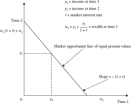
The relation between incomes and wealth is shown in Figure 2.2, with the value of w₁ being given as the intercept on the period 1 axis of the straight line passing through the point (y₁, y₂). If wealth w₁ were all invested at time 1, it would amount to w₂ = w₁(1 + r) at time 2, so the line joining the points w₁ and w₂ must have a slope of − (1 + r). Moreover, any point plotting along the line w₁w₂ in Figure 2.2 has the same period 1 intercept w₁ and thus the same present value. The line w₁w₂ is thus a line of income combinations all having equal present values. Since w₁w₂ goes through the point (y₁, y₂), it follows that the income profile (y₁, y₂) also has present value w₁.

The line w₁w₂ is called the individual's wealth constraint because it defines the maximum present value of different consumption expenditures that can be purchased by spending all available resources. It is also called the market opportunity line because it represents different combinations of funds, available at times 1 and 2, that can be obtained by arranging financial transactions whose net present value is w₁. The entire triangle 0w₁w₂ is called the consumer's opportunity set, because any combination of consumption expenditures lying in or on the triangle is attainable given the consumer's initial wealth. Accordingly, any consumption expenditure pattern the consumer can choose lies within, or on the boundaries of, 0w₁w₂.

2.1.3 Reconciling Preferences with Opportunities

The individual's problem is to choose a pattern of consumption expenditures that maximizes utility given the wealth constraint. The problem can be represented by combining Figures 2.1 and 2.2 as shown in Figure 2.3. If the consumer could not borrow or lend, expenditures would be restricted to the point (y₁, y₂) lying on indifference curve I′ in Figure 2.3. With the ability to make financial transactions, the consumer can move to the higher indifference curve I. In the particular example of Figure 2.3, the consumer will borrow at time 1 and repay = (l + r) at time 2. (The amount repaid is the amount borrowed plus interest.) The amounts expended satisfy the consumer's wealth constraint, as they are required to do. To see this, note that:

may be rewritten as:

or

In other words, the present value of optimal consumption choices is just equal to initial wealth.

FIGURE 2.3 INDIVIDUAL'S CONSTRAINED UTILITY-MAXIMIZING CHOICE OF CONSUMPTION STANDARDS

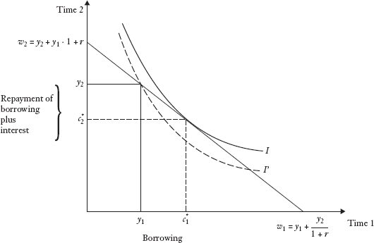
The optimal consumption choices (, ) are found⁵ at the point of tangency between the highest attainable indifference curve and the wealth constraint, where optimal choices mean those the consumer most prefers (among the affordable ones). The spending pattern (, ) will not usually correspond to the consumer's income stream (y₁, y₂). For this reason, the consumer will either borrow (sell a claim against future income) or lend (purchase a claim against future income) through the capital markets thus transferring funds between times 1 and 2 (the slope of the wealth constraint equal to 1 plus the market interest rate).

When the consumer chooses consumption standards optimally, an indifference curve just tangent to the wealth constraint is reached. This is the highest indifference curve the person can reach. This means that at the optimum rate at which the consumer is willing to trade off consumption between times 1 and 2 (the slope of the indifference curve) is just equal to the rate at which the market tells us the market value, at time 1, of $1 to be delivered in period 2. The amount 1/(1 + r) is called the present value of $1 payable at time 2.

The theory of consumers’ financial decisions thus explains that consumers enter into financial transactions to obtain a more satisfactory time profile of consumption expenditures than they could if they merely spent income when received. However, in using the financial markets, they cannot spend more than the present value of their wealth plus future incomes. In a world of certainty, this arrangement means that all consumer lending can and will be repaid; defaults are not permitted. The theory also indicates a consumer is better off if an increment to initial wealth is obtained, because this shifts the wealth constraint to the right. Thus, to leave the consumer as well off as possible, initial wealth should be made as large as possible. This is an important result that we use frequently in the rest of this book.

2.1.4 Numerical Example

In this section we present a numerical example illustrating further aspects of the theory. Consider the following two income streams and a market rate of interest of 10%.

Then

and

In a perfect capital market the consumer will be indifferent between these two income streams because their present values are equal, so that w₁ and are perfect substitutes. This means the consumer can obtain the optimal consumption pattern (, ), also required to have a present value of $1,600, with either income stream. For example, suppose the optimal consumption pattern is ($800, $880), which does have a present value of $1,600 at the assumed 10% rate of interest. If the consumer has the first income stream, $200 is lent at time 1. When repaid with interest at time 2, the loan yields $220. Then expenditure at time 2 can be $880, equal to $660 + $220. If the consumer has the second income stream, $500 is borrowed to finance time 1 consumption, and $550 is repaid at time 2. This leaves $1,430 − $550 = $880 to spend on consumption at time 2.

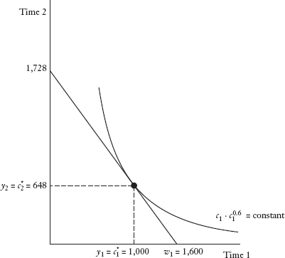
2.1.5 Mathematical Example

The theory can be presented a little more formally by solving a problem like the following one:

subject to y₁ = $1,000, y₂ = $648, and r = 0.08, so that:

Here we have assumed a specific form of the utility function and specific values for incomes and the interest rate, so that we can obtain a numerical answer to the consumption-investment problem. The function c₁c₂^0.6 is the utility function; c₁c₂^0.6 = constant represents the equation of an indifference curve.

The consumer's problem is to maximize utility by finding the optimal consumption pattern (, ) with a present value of $1,600. That is, the solution to the problem must satisfy: ⁶

We can rewrite the last condition as:

Then, substitution into the original maximization problem gives:

A solution to the last problem can be found by setting the derivative taken with respect to c₁ equal to zero. Taking the derivative gives:

We then have:

or

so that

and hence, the solution for time 1 consumption is:

FIGURE 2.4 INCOME AND CONSUMPTION PATTERNS FOR MATHEMATICAL EXAMPLE

Moreover, since

so that

This consumer is atypical in neither borrowing nor lending; that is, the optimal consumption pattern is exactly the same as the income stream. Formally,

A geometrical representation of the problem and its solution is given in Figure 2.4.

2.2 INITIAL WEALTH IS THE ONLY CONSTRAINT ON CONSUMER DECISIONS

It is clear from the foregoing analysis that the wealth constraint keeps the consumer from reaching higher indifference curves. But since this constraint is a line describing combinations of time 1 and time 2 cash flows having equal present values, the analysis also says that the limitation on consumption is entirely reflected by the magnitude of w₁. This is because all cash flow profiles having the same present value leave the consumer with the same opportunities, as we have already argued. We now ask whether these conclusions are altered if either the individual holds durable goods or the capital market is not perfect.

2.2.1 Income and Initial Wealth Combined

We previously mentioned that the consumer might have an initial wealth endowment as well as an income stream. If the initial wealth endowment is in the form of financial assets that can be freely bought and sold in the capital market without payment of transaction costs, their value can be interpreted as included in y₁.⁷

If wealth is in the form of durable goods or other real commodities, we assume they are sold in their respective markets, the proceeds added to current income, and the goods, if needed, rented on a period-by-period basis.⁸ Thus, initially held assets serve only to shift the wealth constraint by the market value of the assets, a movement to the right in Figures 2.2 and 2.3. Hence, the individual's wealth expressed as the present value of the period income stream plus the market value of other initial assets becomes the effective constraint on the choice of consumption patterns over time. Otherwise the analysis is unchanged.

2.2.2 Effects of Capital Market Imperfections

The foregoing analysis showed that individuals in economies with a perfect capital market are never made worse off, and are usually made better off, by their ability to borrow or lend freely in choosing consumption patterns. By implication we can infer that the general level of well-being in such economies is higher than it would be if borrowing and lending were not possible. For these reasons, the presence of capital market imperfections is generally regarded unfavorably. For example, transactions charges such as brokerage fees restrict the amount of initial wealth available and consequently reduce the level of a consumer's well-being. Similarly, other kinds of imperfections such as unequally distributed information can inhibit or even prevent certain financial transactions from taking place.

Although we explore the consequences of market imperfections at length in later chapters, even the simple theory developed so far allows us to develop some conclusions. For example, consider the effects of regulatory constraints that restrict lending. Such an intervention has a potential for leaving at least some individuals worse off, as illustrated in Figure 2.5. Here the individual is affected by a lending restriction that permits borrowing only up to a fixed maximum amount , an amount less than the that would be borrowed if there were no constraint. Thus, the consumer can only attain the consumption standard (), which is tangent to an indifference curve at a lower level of satisfaction than that reached by (, ).

FIGURE 2.5 A LENDING RESTRICTION REDUCING INDIVIDUAL SATISFACTION

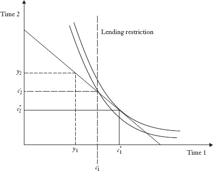
The kinds of lending constraints illustrated in Figure 2.5 are observed in actuality. For example, in times of national emergency, credit restrictions may be justified on grounds of the social benefits they bring through restricting purchases of consumer goods and hence freeing the economy's resources for use in dealing with the emergency. In ordinary times, legislation such as a small loans act sometimes stipulates maximum amounts that individual clients can borrow, a position usually justified on the grounds that some individuals may, if unrestricted, borrow more than is desirable, either for them or society.

2.3 THE MEANING OF THE MARKET RATE OF INTEREST

If we suppose that on balance consumers are net lenders (as is typically the case in developed economies), and if we assume the economy's total borrowing is a given fixed amount, the aggregate supply of credit provided by consumers will determine the market rate of interest. In determining how much to lend, each individual chooses her total consumption expenditures such that the ratio of marginal utilities for consumption at times 1 and 2 is equal to 1 + r, the slope of the market opportunity line. The aggregate of decisions like this will determine the total amount of lending and thus, in turn, the market interest rate. Thus, in a certain sense the market interest rate reflects society's preferences for trading off between consumption at times 1 and 2, respectively.

Moreover, the market interest rate is the reward consumers receive for deferring consumption and is thus the price those demanding funds (e.g., businesses and governments) must pay in order to bid funds away from consumer spending. By paying this price, firms induce saving, which then provides funds necessary for purchasing investment goods. Such investments are worthwhile if they yield a return greater than the market rate of interest, because that means the future consumption made possible by the initial investment will have a higher present value than the consumption originally deferred.

2.4 PRACTICAL IMPORTANCE OF CONSUMPTION-INVESTMENT THEORY

We have seen that most households will be better off in economies with smoothly working financial markets. A practical circumstance reflecting the theory's predictions is that many householders make contributions to pension funds; that is, by saving (and hence lending to others) they are able to arrange a more satisfactory profile of anticipated consumption expenditures than would be available if there were no such arrangements.

Household investment decisions are important to firms in real-world economies because households are the primary source of finance capital; that is, in most developed economies households are on balance net lenders. Most of these household funds are in financial institutions like life insurance companies and pension and mutual funds. The funds raised by these institutions are reinvested in corporate and government securities. Households also make some direct purchases of corporate and government securities, thus acting directly as lenders to business and government. Households’ desires to finance future consumption thus provide the main source of funds that firms can use to finance their investment activities.⁹ The price firms must pay for these funds is the price that households require to defer present consumption until some future time.

The theory developed so far provides a criterion for managers of firms. In a certainty world with a perfect capital market the only constraint on consumer decisions is wealth, and the greater the wealth, the greater the consumer satisfaction. Accordingly, the best that management of corporations can do for their owners is to maximize the present value of their ownership interests in these corporations. That is, management's task is to create as much wealth as possible, which is what all the owners of firms require their management to do. Management performs its wealth creation task by reinvesting funds raised at rates higher than the market rate of interest. In the next chapter we turn to the details of how management performs this task.

KEY POINTS

• The behavior of consumers as both demanders of goods and services and as suppliers of funds to the capital market is important in developed economies.
• The theory of consumer choice examines the trade-offs and decisions consumers make in their purchase decisions. The preference of consumers is expressed in their utility functions.
• It is assumed that consumers operate in a perfect capital market in which: (1) there are many transactors, and no single transactor is large enough to affect prices or interest rates; (2) the same (certain) information about market prices and the relevant terms of any transaction are available to all parties; and (3) there are no costs of transacting other than the ruling market rate of interest.
• In a perfect capital market there is no need for borrowers to borrow at a rate in excess of the market interest rate or for lenders to provide credit at a rate below the market interest rate.
• Preferences of consumers can be expressed mathematically by means of a utility function where equally satisfactory consumption patterns are depicted as points on an indifference curve.
• The marginal rate of substitution between present and future consumption is the slope of an indifference curve at any point and indicates the consumer's preference for trading off consumption at the present time against consumption in the future.
• The value of available assets at a given time consists of the market value of stocks of real durable goods and financial assets carried over from previous periods.
• The theory of consumers’ financial decisions explains that consumers enter into financial transactions to obtain a better time profile of consumption expenditures than they could by spending their entire income at each time point when it is received.
• A perfect capital market means consumers can never be worse off by having the freedom to borrow or to lend. This result implies that capital market imperfections are regarded as unfavorable.
• Capital market imperfections include transactions charges, unequally distributed information, and regulatory constraints.
• As each consumer decides how much to lend or borrow, the aggregate of consumer decisions will determine the total amount of lending or borrowing and thus in turn the market interest rate. The market interest rate is the reward consumers receive for deferring consumption and is thus the price those needing funds must pay in order to bid funds away from consumers spending funds in a given period.

QUESTIONS

1. a. What are the implications for credit risk in a perfect capital market under circumstances of certainty?

   b. In a perfect capital market, would an entity in need of funds pay an interest rate in excess of the market interest rate? Why or why not?

2. Why is financial decision making made easier in a perfect capital market?
3. a. What is meant by a utility function?

   b. What is an indifference curve?

   c. What is meant by the marginal rate of substitution between present and future consumption?

4. Draw a line of equal present values for the cash flow profile of $100 now and $210 next period, interest rates at 5%. What is the maximum amount that can be realized in the first period if, in addition to interest charges, 1% commission is collected from the proceeds of any borrowings? Show the effect of the commission on your graph, and explain the importance of this exercise for the consumer's well-being.
5. Suppose interest rates are zero and the consumer's utility is u(c₁, c₂) = (c₁, c₂), while the two incomes are (y₁, y₂) = (75, 125). Find the optimal consumption in each period, and also indicate what financial transactions the consumer makes. Show the answers on a diagram.
6. Suppose an investment of $40 now will return $110 one period later, interest rate 10%. Then:

   

   In a perfect market the owner of such an income stream can create any cash flow profile that satisfies:

   

   Hence, if this person is offered another investment opportunity that costs $10 now but pays $77 one period later, it is as satisfactory as the first. Why might this reasoning not work if there were a 1% brokerage charge on amounts borrowed?

7. a. Use a diagrammatic analysis to show why a consumer facing a two-period planning problem under certainty may benefit from the existence of a capital market. Explain the different features of your diagram, and list important assumptions of your analysis (other than those already mentioned).

   b. Use a similar diagram to show why some individuals would be worse off if (in the world described in part a) lenders restricted the amount an individual could borrow to a fixed percentage of his current (first-period) income.

   c. Might such a restriction be a good policy in the real world? Why or why not?

8. Is it possible to say anything, on the basis of the certainty theory of consumption-investment decisions, about whether consumers will borrow more (less) as interest rates rise? Why? Use a diagram.
9. Try to explain why an investor might be indifferent between dividends (cash payments at time 1) and capital gains (cash payments at time 2) in a certainty world with a perfect capital market and no taxes. The proposition means that a change in dividends is offset by a change in capital gains having the same present value. Use a diagram, clearly labeled, and keep your explanations as short as possible.
10. A consumer's consumption-utility function for a two-period horizon is ; the income stream is y₁ = 2,000; y₂ = 1,296; and the market rate of interest is 0.08. Determine values for c₁ and c₂ that maximize utility. Is the consumer a borrower or a lender?
11. In a two-period problem, a consumer whose preferences satisfy the assumptions of this chapter will consume more of at least one good as income rises. True or false? Show diagrammatically why your answer is correct.
12. Show diagrammatically how an individual earning income at time 1 could provide for consumption at time 2, where time 2 represents retirement and no income is earned.
13. Explain whether you agree or disagree with the following statement: In a perfect capital market, individuals are made worse off by their ability to borrow or lend freely in choosing consumption patterns.
14. What is meant by a capital market imperfection? Give two examples.