12

ON CHOOSING RISK MEASURES

As we explained in the previous chapter, risk-management problems can be viewed as problems aimed at optimizing a variety of criteria.¹ In this chapter, we examine how risk measures are defined and used to help select solutions to the risk-management problems of either individual or institutional investors. There are many different risk measures, but their use is based on the same considerations: Each measure attempts both to describe risks and to provide some information for solving risk-management problems. However, since any risk measure gives a summary description of lottery characteristics, it can only be used correctly in the context of particular optimization problems, as we show in this chapter.

12.1 USING RISK MEASURES

A risk measure is a function, denoted by ρ, that maps lotteries X into the set of real numbers R:²

ρ: X → R

The function ρ is defined to have a positive range. For example, if a risk management problem is formulated as maximizing an expected utility function u, and if u has a positive range,³ then:

ρ(X) ≡ m − E[u(X)]

where m is an appropriately large positive constant, could serve as a risk measure. While this observation shows how risk measures are related to risk-management problems, it is not very informative because it simply restates the original problem. Fortunately, there are several other approaches to finding helpful measures, as we demonstrate in the balance of this chapter.

12.1.1 Measures Based on the First Two Moments

Financial economics has traditionally focused on using the mean and the variance of probability distributions as descriptive risk measures, in part because these two measures address the essence of expected utility maximization when the utility function is concave. Consider such a utility, and suppose further, for explanatory purposes, that the risk-averse investor faces lottery X with the following two outcomes (referred to as two-point lotteries) and probability distribution:

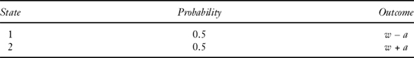
Based on the above, E(X) = w and σ²(X) = a², where σ² (X) is the variance of the above two-point lottery outcomes. If a increases while the lottery's expected value remains constant, it is easy to show that the certainty-equivalent value of X (see Chapter 11) will decrease for any risk-averse decision maker. That is to say, among symmetric two-point lotteries having equal expected values but differing variances, the risk-averter will prefer the one having the smallest variance.⁴

Thus, we may say, at least for these special kinds of lotteries,⁵ that expected utility decreases as variance increases (holding expected value constant), and expected utility increases as E (X) increases (holding variance constant). Expected payoff is a measure of expected future wealth,⁶ while variance of payoffs is a measure of wealth dispersion. Moreover, in these cases we can use either the variance σ²(X) or the standard deviation σ (X) as risk measures, since either describes the lottery's dispersion. It is equally possible to use other measures of dispersion such as mean absolute deviation, defined by:

E[|X − E(X)|]

Selection among dispersion measures is largely a matter of reflecting significant problem characteristics. For example, the mean absolute deviation measure, defined above, gives less weight to extreme outcomes than does the variance.

Prior to the development of Markowitzian portfolio theory (see Chapter 13) the effects of risk were recognized by using a discount factor of the form 1/(1 + r + π), where r represents the risk-free rate of interest and π a risk premium that is positive for valuations made by risk-averters. Markowitz proposed determining the risk premium more nearly exactly by using variance of return on the entire portfolio as a measure of risk.⁷ Markowitz noted that covariances between pairs of individual investments (i.e., linear correlation coefficients) can be used to examine the effects of diversification on the variance of portfolio return. Markowitz thus explained that diversification is a solution property emerging from calculating the portfolio variance of return.

The Markowitz approach can be used correctly with some distributions and some utility functions. The mean-variance trade-offs described by Markowitz exactly characterize solutions to any expected utility maximization problem whose random returns are jointly normally distributed, and also to quadratic utility maximization problems even if returns are not normally distributed. In both these cases, ρ(r_X) ≡ σ²(r_X) or ρ(r_X) ≡ σ(r_X) serve as risk measures that correctly rank portfolios constrained to have the same expected return. Of portfolios with the same expected return, a minimum variance portfolio is preferred. Alternatively, expected return can be used to rank portfolios constrained to have the same variance; in this case a maximal return is sought.⁸ Portfolios that offer the best available combinations of mean and variance are said to lie on a mean-variance efficient frontier.

Two of the main pricing models in current use, the theoretically oriented Capital Asset Pricing Model (CAPM) and the empirically oriented Arbitrage Pricing Theory (APT), frequently describe return distributions using their first two moments⁹—expected value (mean) and variance. The return variance of the portfolio is then readily related to the return variance of its component securities. For example, if a portfolio is composed of two securities, its risk as assessed by the CAPM is described using:

σ²(r_X) r_Y) = σ²(r_X) + σ²(r_Y) + 2σ(r_X) σ(r_X) corr(r_X, r_Y)

where

corr(r_X, r_y) ≡ E{[r_X − E(r_X)][r_Y − E(r_Y)]}

is the linear correlation coefficient between r_X and r_y.

Given either normally distributed random variables or quadratic utilities (or both), desirable risk-return trade-offs can be easily calculated using a solution property known as two-fund separation. For example, if there is a risk-free asset, the optimal portfolios described by the CAPM are weighted combinations of the risk-free asset and the market portfolio.¹⁰

Recent research has identified the class of random variables for which it is theoretically correct to use linear correlation as a dependence measure—the class of distributions whose equidensity surfaces are ellipsoids. This class of so-called elliptical distributions includes both the normal distributions and the Student t-distributions with finite variances.¹¹

12.1.2 Measures Recognizing Higher Moments

As explained in the previous chapter, empirically estimated return distributions from real-world financial markets are not usually elliptical—rather they are heavy-tailed, skewed, and have kurtosis measures E[X − E(X)]⁴ different from that of the normal distribution.¹² In addition, some empirically estimated distributions may have extreme outcomes that occur with significantly larger probability than even some choices of heavy-tailed distributions will reflect. A linear correlation coefficient may not correctly describe the dependence between the risks of individual random variables having empirically estimated distributions, and risk-return rankings derived from the CAPM may not correctly characterize solutions to the associated utility maximization problems.¹³

In particular, using a variance-covariance model for non-elliptical distributions can lead to severe underestimates of extreme losses. The difficulties are compounded by the fact that higher moments such as kurtosis can be unstable and must therefore be estimated from relatively large samples. Moreover, it is not known how many parameters are actually necessary to identify a multiparameter efficient frontier.¹⁴ Still further, even if the relevant optimization problems could define optimal choices for a whole class of investors, the problems can be computationally too complex to be solved for large portfolios, and the computational difficulties increase still further if short sales are prohibited.¹⁵ On the other hand, if the optimization problem is simplified to make it computationally more tractable, then only a subset of optimal portfolios will be identified, no matter what risk measure is chosen.

12.2 MEASURES OF RISKINESS

We turn now to considering risk measures with broader application than mean and variance. This section examines two such measures, the Aumann and Serrano (2008) measure of riskiness and a related measure proposed by Foster and Hart (2008). The Aumann-Serrano measure extends the ranking capabilities of measures based on mean and variance, and of those based on stochastic dominance. Further, the Aumann-Serrano measure provides relations between the riskiness of portfolios and their component securities for arbitrary forms of distributions. It is both a global description of lottery riskiness and related to the Arrow-Pratt measures of local risk aversion explained in Chapter 11.

The Foster-Hart measure is another global description of a lottery's riskiness and is also related to the Arrow-Pratt measures of local risk aversion. However, it is based on a criterion of bankruptcy avoidance, a postulate different from the axioms underpinning the Aumann-Serrano measure.

The next section states the two axioms¹⁶ on which the Aumann-Serrano measure is based and then discusses the measure's main properties. The conceptual underpinnings and purposes of the Aumann-Serrano measure are next compared briefly with the underpinnings and purposes of the related riskiness measure proposed by Foster and Hart (2008).

12.2.1 Aumann-Serrano Axioms

A lottery X is said to be riskier than a lottery Y if ρ*(X) ≥ ρ*(Y), where ρ*() denotes Aumann-Serrano (2008) riskiness. As will be shown shortly, the function ρ*() is defined uniquely by a pair of axioms, referred to as the duality axiom and the positive homogeneity axiom, respectively. To do so, however, it is first necessary to introduce the concept of “uniformly more risk averse,” a stronger condition than Arrow-Pratt risk aversion. A utility function u_i is said to be more risk averse than a utility function u_j if r_Ai(w) ≥ r_Aj(w) for some w, where r_Ai(.) is the Arrow-Pratt measure of absolute risk aversion (see Chapter 11). Aumann-Serrano's stronger condition is as follows. If:

min_w[r_Ai(w)] ≥ max_w[r_Aj(w)]

for all levels of wealth w, then i is said to be uniformly more risk averse than j, while if:

max_w[r_Ai(w)] ≥ min_w[r_Aj(w)]

for all levels of wealth w, then i is uniformly less risk averse than j. The concepts of uniformly more (less) risk averse mean that one function's measure of risk aversion is no less (no more) than that of another across the measures’ entire domain. “Uniformly risk averse” is therefore a partial ordering¹⁷ since it does not characterize relations between measures of risk aversion that can cross each other.

We can now state the axioms on which the Aumann-Serrano measure is based. The first, the duality axiom, refers to two agents, one uniformly more risk averse than the other, and two lotteries, one riskier than the other.

Duality axiom: If u_i (w) is uniformly more risk averse than u_j(w), if ρ*(X) ≥ ρ*(Y), and if i accepts X at wealth level w, then j accepts Y at w.

The duality axiom stipulates that if the uniformly more risk-averse agent accepts the riskier of the two lotteries, the uniformly less risk-averse agent will accept the less risky lottery.¹⁸

The second axiom, positive homogeneity, axiom refers to the scale of a lottery.

Positive homogeneity axiom: ρ*(t X) = tρ*(X) for all positive numbers t.

This axiom says that changing the scale of a lottery will change the risk measure similarly. For example, if a lottery has outcomes measured in thousands of dollars and a risk measure of, say, 7, then measuring the same lottery in hundreds of dollars will produce a risk measure of 10 × 7 = 70. In particular, the positive homogeneity axiom means that if one has a riskiness measure for a lottery whose payoffs are measured in dollars, it will be easy to convert both the lottery and the risk measure to reflect payoffs measured in rates of return. The positive homogeneity axiom is also useful in establishing relations between portfolio riskiness and the riskiness of the individual securities composing it.

The next theorem defines the riskiness measure.

Theorem 12.1. If the duality and positive homogeneity axioms are satisfied, then for any lottery¹⁹ X, ρ*(X) is uniquely defined as the solution to:

The proof of Theorem 12.1 is provided in Aumann-Serrano (2008). A practical way of calculating ρ*(.) is given in the Section 12.2.2, along with several other examples illustrating the measure's properties.

Note that the function in Theorem 12.1 represents the preferences of a decision maker whose utility function is:

with risk-aversion parameter γ = 1. Equation (12.2) displays a constant absolute risk-averse utility function,²⁰ and if γ = 1, then r_A(w) ≡ −u″(w)/u′(w) ≡ 1 for all w.

It follows from the next theorem that ρ*(.) permits comparing the riskiness of lotteries for all decision makers who are uniformly more risk averse than the decision maker in equation (12.2).

Theorem 12.2. If ρ*(X) ≥ ρ*(Y), then Y is weakly preferred to X for all decision makers who are uniformly more risk averse than a decision maker whose utility function is constant absolute risk averse with a risk-aversion parameter γ =1.

Again, the proof may be found in Aumann-Serrano (2008).

As an example of Theorem 12.2, a decision maker who is constant absolute risk averse with a risk-aversion parameter of 1.3 is uniformly more risk averse than the decision maker in equation (12.2), and hence, ρ*(X) ≥ ρ*(Y) indicates that the decision maker with a risk-aversion parameter of 1.3 (weakly) prefers Y to X, just as does the decision maker with a risk-aversion parameter of 1.

The results can be further extended to other uniformly more risk-averse decision makers. However, although such comparisons are valid for any decision maker who can be described as uniformly more risk averse than the decision maker in equation (12.2), there can still be other decision makers who are not uniformly more risk averse and for whom the comparison will not be valid. That is why the Aumann-Serrano measure is a partial rather than a complete ordering.

12.2.2 Properties of ρ *()

Theorem 12.1 shows that ρ*() relates a lottery's global riskiness measure to the local definition of absolute-risk aversion. Formally, ρ*() is continuous, subadditive (as defined below), and consistent with dominance orderings. (Consistency is discussed in Section 12.3.) Both the form of ρ*(.) given in equation (12.1) and the following examples show that riskiness is more sensitive to the loss side of a lottery than to its gain side. Other useful properties of ρ*() are also illustrated by the examples.

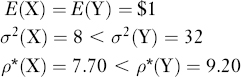
To see that ρ*(.) recognizes the effects of both mean and dispersion, we consider three lotteries. First, compare a lottery X that offers either a payoff of $5 or a loss of $2 with equal probability to a second lottery Y that offers a payoff of $4 or a loss of $3, also with equal probability. Then:

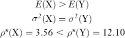
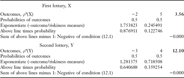
The calculations to find ρ*(X) and ρ*(Y) can be performed in an Excel spreadsheet as illustrated in Table 12.1. The table shows how to set up the spreadsheet to incorporate each lottery's outcomes and probabilities, as well as how to calculate the expected utilities. This involves exponentiation of each outcome [divided by a tentatively chosen value for ρ*()], then multiplying the result by the relevant probability. Then, for the specified value of ρ*(), the table shows further how to check whether equation (12.1) is satisfied by the just-calculated expected utility measure. If the solution condition is not satisfied for the initially chosen value of ρ*(), then that value is successively increased or decreased until a solution is converged upon.²¹ Usually only a few values need to be tried before a solution is found.

TABLE 12.1 CALCULATING RISKINESS MEASURES

Continuing to explore how ρ*(.) incorporates the effects of both mean and variance, next consider a lottery Z that offers a payoff of $6 or a loss of $3 with equal probability. Then:

²²

Notice that the foregoing examples weigh both the effects of changing mean in comparing lotteries X and Y, and the effects of changing variance in comparing lotteries X and Z. Clearly, the riskiness measure can quantitatively recognize the effects of changing mean and changing variance simultaneously, thus in effect defining a function whose domain of definition can be taken as mean-variance space. Since each point in mean-variance space can be associated with a value of the riskiness measure for a given family of distributions,²³ the measure constitutes an advance over historical mean-variance methods that cannot assign a quantitative measure to changing both mean and variance simultaneously.²⁴ Essentially, the simultaneous effects are recognized by the expected utility maximization calculation used to define ρ*(.) [recall equation (12.1)].

Aumann and Serrano (2008) also show that the riskiness measure is defined exactly for normally distributed variables. If X is normally distributed:

ρ*(X) ≡ σ²(X)/2E(X)

Consequently, the riskiness of any normally distributed variable X can be compared to an equivalently risky standardized form of normal distribution N. For example, take E(N) = 1 and σ²(N) = 2ρ*(X). Then N[1; 2ρ*(X)] (where the first argument of N refers to its mean and the second to its variance) has the same riskiness as X. It follows immediately that if X and Y are both normally distributed and ρ*(X) < ρ*(Y), then N[1; 2ρ*(X)] is less dispersed than N[1; 2ρ*(Y)].

Aumann and Serrano also offer another and more widely applicable benchmark for ρ*(.). Suppose X is a lottery, no longer restricted to be normally distributed, such that ρ*(X) = k. Then the lottery B having outcome −k with probability 1/e where e²⁵ is 2.17828 and therefore, its reciprocal is approximately equal to 0.37, and a sufficiently large²⁶ outcome m with probability 1 − 1/e, approximately 0.63, has ρ*(B) = k. That is, every lottery with a given riskiness measure can be compared to a standard lottery that offers (1) a loss equal to the riskiness measure k (realized with probability 1/e) and (2) a gain equal to some large outcome realized with probability 1 − 1/e. Both the original lottery and the benchmark have the same riskiness measure k.

The riskiness measure also helps to relate a portfolio's riskiness to the riskiness of the securities composing it. For any lotteries X and Y:

ρ*(X + Y) ≤ ρ*(X) + ρ*(Y)

That is to say, the riskiness of a sum of lotteries is no greater than the sum of the riskiness measures for the individual lotteries. This property is known as subadditivity. Moreover, if the variables X and Y are independent and identically distributed, then not only is ρ*(X) = ρ*(Y) but also:

ρ*(X + Y) = ρ*(X) = ρ*(Y)

That is, ρ*(.) does not increase when the two independently distributed variables are added together. Still further, if X and Y are totally positively correlated (i.e., if they are the same lottery), then:

ρ*(X + Y) = 2ρ*(X) = 2ρ*(Y)

Finally, if the two variables are totally negatively correlated (e.g., if X ≡ −Y), then ρ*(X + Y) is minimized, although it need not equal zero.²⁷

Applying the positive homogeneity property to the above statements provides immediate portfolio theoretic applications. Let w and 1 − w be positive weights. Then for any²⁸ X and Y:

ρ*(w X + (1 w)Y) ≤ wρ*(X) + (1 − w)ρ*(Y)

the riskiness of the portfolio does not exceed the weighted riskiness measures of its components. Still further, the riskiness of an equally weighted sum of independent and identically distributed lotteries decreases:

ρ*(X/2 + Y/2) = ρ*(X)/2 = ρ*(Y)/2

Thus, ρ*(.) provides natural generalizations of insights developed by Markowitzian portfolio theory.

The riskiness measure can also be applied to compound lotteries. For example, if X and Y are compounded with probabilities p and (1 − p), respectively, and if ρ*(X) ≤ ρ*(Y), then Aumann and Serrano (2008, p. 819) show that:

ρ*(X) ≤ ρ*(p X + (1 − p)Y) ≤ ρ*(Y)

A compound lottery (a lottery of lotteries) has a riskiness measure that lies between the riskiness measures of the individual lotteries making up the compound lottery.

Finally, to show that ρ*(X) does not always reflect all aspects of a lottery's desirability, Aumann and Serrano (2008, p. 823) compare a lottery X, with equally probably payoffs $5 and −$3, to a lottery Y having payoffs $15 and −$1 with probabilities 1/8 and 7/8, respectively. Note that:

However, even though Y has the greater riskiness, it is possible to find constant absolute risk-averse utility functions u with risk-aversion parameters²⁹ for which E[u(Y) ≥ E[u(X)]. The example shows not only that the riskier lottery is more desirable for some decision makers, but also shows once more that the ranking provided by ρ*(.) is a partial ordering.³⁰ In this example, it does not rank the lotteries similarly for all decision makers, but only for those who can be ranked as uniformly more risk averse. As with other measures, it is necessary to know the limitations of ρ*(.) in order to use it correctly.

12.2.3 Foster-Hart Operational Measure

Foster and Hart (2008) acknowledge the inspiration of Aumann and Serrano (2008) in developing their own operational measure of riskiness. The Foster-Hart measure shares many properties with the Aumann-Serrano measure, and quite often yields very similar rankings. For these reasons we shall not present the Foster-Hart measure's details, but it is still important to note the following. The Aumann-Serrano measure is derived from critical levels of risk aversion and is concerned principally with comparing lotteries’ riskiness, while the Foster-Hart measure is derived from critical levels of wealth and is defined separately for each lottery. Foster-Hart develop their measure using only a single assumption: that no bankruptcy is preferred to bankruptcy.³¹ They also show how their measure is related to Arrow-Pratt constant relative risk-averse utilities. Foster-Hart further stress their measure's practicality, meaning that it may find use in institutional portfolio choice problems. In particular, the measure can be used to tell when lotteries should be rejected. However, it does not otherwise help with the optimal portfolio selection problem—a limitation similar to many of the other measures discussed in this chapter.

12.3 CONSISTENT RISK MEASURES AND STOCHASTIC ORDERINGS

The concept of consistency describes a further link between utility-maximizing portfolios and risk measures. Recall that dominance criteria were introduced in Chapter 9. This chapter will further discuss these dominance criteria and demonstrate how each is consistent with utility maximization for a given class of decision makers.

A risk measure ρ(.) is said to consistent with a stochastic-order relation if E[u(X)] ≥ E[u(Y)] for all utility functions u belonging to a given category³² implies that ρ(X) ≤ ρ(Y) for all admissible lotteries X ≤_D Y, where ≤_D indicates a particular dominance relation. Since consistency can characterize the set of all optimal portfolio choices when either wealth distributions or expected utility satisfy the conditions summarized by a particular order relation, it is useful to examine how consistency can be used with the dominance criteria introduced in Chapter 9 and defined further below. It will be shown that ρ*(.) extends the orderings provided by each of the dominance criteria.

12.3.1 First-Degree Dominance

One form of stochastic dominance that we will describe here is first-degree stochastic dominance, which orders a subset of all possible lotteries for all nonsatiable agents. Denote by U₁ the set of all utility functions representing nonsatiable agents; that is, the set containing all nondecreasing utility functions. We say that X dominates Y in the sense of the first-degree stochastic dominance (FSD), denoted by X ≥_FSD Y, if a nonsatiable agent weakly prefers X to Y. In terms of expected utility, X ≥_FSD Y E[u(X) ≥ E[u(Y)], for any u ∊ U_1.m. Formally, the first-order dominance relation is characterized by Theorem 12.3, showing that the test for FSD involves comparing cumulative probability distributions for lotteries.

When the conditions of Theorem 12.3 are satisfied, FSD gives a consistent ranking for all nonsatiable decision makers: X ≥_FSD Y if and only if E[u(X)] ≥ E[u(Y)] for all nondecreasing utility functions u ∊ U₁. Moreover, ∊*(.) extends the partial ordering provided by FSD. For example: ³³

If X ≥_FSD Y, then ρ*(X) ≤ ρ*(Y)

To illustrate, suppose X is a lottery that offers either $3 or −$2 with equal probability; Y a lottery that offers either $3.2 or −$1.8 with equal probability. Clearly, X ≥_FSD Y. Moreover, ρ*(Y) is approximately $12.20, while ρ*(X) is approximately $6.05.

The condition E(X) ≥ E(Y) is necessary³⁴ for X ≥_FSD Y. On the other hand, ranking by means is not sufficient for FSD. If E(X) ≥ E(Y), it does not necessarily follow that every nonsatiable agent would necessarily prefer X. In effect, there can be nonsatiable agents who would choose X and other nonsatiable agents who would choose Y.

First-degree stochastic dominance is a relatively restrictive partial ordering that is only capable of ranking lotteries whose distribution functions do not cross at any point in their respective domains. It is possible to rank more lotteries by imposing additional restrictions on agent preferences.

12.3.2 Second-Degree Dominance

We introduced the idea of second-degree stochastic dominance in Chapter 9. Denote by U₂ the set of all utility functions that are both nondecreasing and concave. Thus, U₂ represents the set of nonsatiable risk-averse agents, and U₂ is contained in U_1. We say that a lottery X dominates lottery Y in the sense of second-degree stochastic dominance (SSD), denoted by X ≥_SSD Y, if a nonsatiable risk-averse agent weakly prefers X to Y. In terms of expected utility, SSD is also a consistent ordering:

X ≥_SSD Y E[u(X) ≥ E[u(Y)] for any u ∊ U₂

For example, consider a lottery Y with two possible payoffs—$100 with probability ½ and $200 with probability ½, in comparison to a lottery X yielding $180 with probability one. A nonsatiable risk-averse agent would never prefer Y to X because the expected utility of Y is not larger than the expected utility of X:

E[u(X)] = u(180) ≥ u(150) ≥ u(100)/2) u(200)/2 = E[u(Y)]

where u (x) is assumed to be nondecreasing.

The test for SSD is an integral test.

Theorem 12.4. X ≥_SSD Y if and only if

for all a in the (assumed common) domain of F(x), F(y).

Similar to the result of the previous section, ρ*(.) extends the partial orderings provided by SSD. For example: ³⁵

If X ≥_SSD Y, then ρ*(X) ≤ ρ*(Y)

To illustrate, suppose Y is a lottery that offers either $2 or −$1 with equal probability; X offers either $2.10 with probability 0.27, $1.95 with probability 0.23, and −$1.00 with probability 0.5. Clearly, X ≥_SSD Y. Moreover, ρ*(X) is approximately $2.071, while ρ*(Y) is approximately 2.075.

As it is with FSD, E(X) ≥ E(Y) is a necessary condition for SSD. However, in contrast to FSD, the integral condition for SSD is less restrictive in that, as long as equation (12.3) is satisfied, the distribution functions may cross each other.

12.3.3 Rothschild-Stiglitz Dominance

As first mentioned in Chapter 9, Rothschild and Stiglitz (1970, 1971) introduce a dominance ordering that requires agents be risk averse, but not necessarily insatiable. The class of risk-averse agents considered is represented by the set of all concave utility functions, a set that contains U₂. The class of random variables ranked by Rothschild-Stiglitz dominance (RSD) is restricted to have the same expected values.

In practical terms RSD and SSD both focus on dispersion, but RSD provides economic insight that is not stressed in the development of SSD. In particular, RSD means that a dominated variable can be written as the sum of a dominating variable plus noise terms with a mean³⁶ of zero; that is, the dominated variable is more dispersed than the dominating variable. Like FSD and SSD, RSD provides a consistent ordering.

As mentioned in the previous sections, ρ*(.) extends the partial orderings provided by dominance relations. In the present case:

If X ≥_RSDY, then ρ*(X) ≤ ρ*(Y)

as established in Aumann and Serrano (2008, p. 818); the riskiness measure is also consistent with RSD.

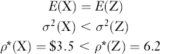
To illustrate, recall an example that has already been investigated. Let X offer either $5 or −$2 with equal probability, and Z offer $6 or −$3 with equal probability. Then:

12.3.4 Generalizations and Limitations

Dominance orderings are partial rankings, each capable of ranking only a subset of all possible portfolio choices. Nevertheless, successively restricting the set of preferences expands the class of portfolios that can be ranked by a given ordering. For example, SSD ranks more random variables than FSD, but does so for a subset of U₁.³⁷ On the other hand, finding portfolios that satisfy a dominance ordering is not always a trivial computational task, especially if the portfolio can contain many financial instruments with different forms of return distribution. Thus, risk measures based on dominance orderings provide only a partial solution to the problems of selecting optimal portfolios.

Given a class of investors, consistency implies that all the best investments for that class are among the dominating, and therefore the less risky, ones. However, there is no guarantee that the less risky choices are utility maximizing choices when all possible portfolios are considered. For example, the decision maker might find that some portfolio, not capable of being ranked by a given stochastic ordering, could offer a higher expected utility.

12.4 VALUE AT RISK AND COHERENT RISK MEASURES

In this section we first consider a measure known as Value at Risk, usually referred to as VaR. VaR has been and is still widely used in practice and has also been endorsed by bank regulators. However, the use of VaR has also been criticized severely by academics.³⁸ The section will first discuss the properties of VaR, then the difficulties its use presents. We next consider an axiomatic approach to defining risk measures, developed by Artzner, Delbaen, Eber, and Heath (1999), henceforth ADEH. ADEH developed the concept of coherent measures as a way of resolving some of the difficulties with VaR, and we show below how the choice of coherent measures can be regarded as superior to the choice of VaR measures. In so doing, we also compare and contrast the properties of coherent measures with the concept of Aumann-Serrano riskiness.

12.4.1 Value at Risk

VaR, originally developed by JPMorgan in the 1980s, defines the minimum amount of money a portfolio manager can expect to lose with a given probability. As an example, consider a portfolio whose possible value at the end of a 30-day period beginning now can be regarded as a normally distributed random variable with an expected value of $20 million and a standard deviation of $2 million. Then, given the normality assumption, the probability that this portfolio will finish the 30-day period with a realized value of $17 million or less is 0.0668. In VaR terms,³⁹ this situation would be expressed as a VaR of $3 million with a probability of 0.0668.

In other words, VaR states a loss magnitude that defines the upper limit of a probability distribution's lower tail. However, some important qualifications need to be kept in mind. First, the probability of 0.0668 implies that the portfolio manager could well realize a loss of more than $3 million, because VaR refers only to the tail's upper boundary. Second, the normal distribution used is quite likely to be an approximation of the actual distribution. In practice, portfolio losses of $3 million or more may actually have a probability distribution that is non-normal, with a fatter lower tail (as well as a fatter upper tail) than that of the normal distribution. This means that in practice the probability of losing $3 million or more is likely to be higher than 0.0668. (See Web-Appendix M for a discussion of alternative probability distributions.)

Despite the foregoing qualifications, VaR has been widely used by both portfolio managers and banks as a measure of the risks they face. Although the suitability of VaR is really restricted to business-as-usual periods, VaR measures have also sometimes been relied on in turbulent periods. In practice, VaR calculations are often based on data from the preceding three or four years of business. Hence, if business has operated smoothly for that period, VaR may well understate the dangers of future loss. Indeed, VaR measures based on loss experience during past business-as-usual periods may not even be very useful for predicting future losses in a changed economic environment, and portfolio managers using VaR have sometimes failed to ask what kinds of losses might be incurred if the assumptions underlying their calculations were to change.

There are still other practical problems with VaR. Attempts to apply VaR to non-elliptical return distributions ignore information contained in the tail of the distribution; that is, VaR ignores extreme events. In addition, attempts to reduce portfolio VaR may actually have the effect of stretching out the tail of losses, increasing the magnitude of losses that might be realized in extreme cases. Still further, portfolio diversification may both increase the risks assumed and prevent adding up component VaRs. Moreover, VaR can be unsuitable for use in many optimization problems, especially if the VaR measure has many local extremes that make rankings unstable. Finally, VaR can provide conflicting results at different confidence levels.

The use of VaR can also create such system problems as the dynamic instability of asset prices. Episodes of volatility increase VaR, which in turn triggers moves to sell, creating still further volatility. Fair-value accounting, which requires assets to be valued at current market prices, also accentuates price movements because marking assets down to lower market prices can stimulate further selling. Despite the foregoing problems, and even though the use of VaR has sometimes led to disastrous results, it still finds favor with regulatory agencies.

VaR has also come under severe criticism for theoretical reasons. First, VaR is not subadditive unless the joint distribution of returns is elliptical. But in the case of elliptical joint distributions, a VaR-minimizing portfolio is also a Markowitz variance-minimizing portfolio, meaning that VaR is no better than the simpler and more traditional variance measure. Finally, VaR is not a coherent measure in the sense discussed in the next section.

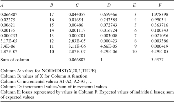
But if the decision maker accepts the four coherence axioms presented in the next section, both conditional VaR (CVaR)—a modification of VaR that more carefully takes into consideration tail risk—offers possible choices of measure that does not suffer from the same problems.⁴⁰ In particular, a switch from VaR to CVaR essentially requires calculations similar to those used for VaR. In the example at the beginning of this section, CVaR is the conditional expected value of losses described by the tail limit of $3 million, and is clearly a number larger than that $3 million. Since conditional losses are at least $3 million, the appropriate value for CVaR is in fact roughly equal to $3.47 million.⁴¹

12.4.2 Axioms for Coherent Risk Measures

As just mentioned, the concept of coherent measures was developed in an attempt to remedy the deficiencies of using VaR. Artzner, Delbaen, Eber, and Heath (1999, henceforth ADEH) define coherent risk measures as measures that conform to the following four axioms.

Positive homogeneity: ρ(tX) = tρ(X) for all random variables X and all positive real numbers t.

That is, the scale of the risk measure should correspond to the scale according to which the random variables are defined. Recall that positive homogeneity is also one of the two principal axioms used by Aumann-Serrano (2008).

Subadditivity: ρ(X + Y) ≤ ρ(X) + ρ(Y) for all random variables X and Y. Subadditivity insures that combining random variables cannot increase a risk measure beyond the sum of the measures for individual components.

Subadditivity is assumed by ADEH, whereas this chapter showed earlier that it follows as a consequence of the Aumann-Serrano axioms.

Monotonicity: X ≤ Y implies ρ(Y) ≤ ρ(X) for all random variables X and Y.

The monotonicity axiom rules out any asymmetric form of measure, and for that reason, cannot represent all decision makers. Moreover, monotonicity is not postulated by Aumann and Serrano, and indeed their measure is more sensitive to the downside of a lottery than to its upside. Furthermore, monotonicity rules out measures such as the semi-variance,⁴² which deals only with downside risk.

Translation invariance: ρ(X + k) = ρ(X) − α for all random variables X, all certainty outcomes k, and all real numbers α. Translation invariance implies that adding a sure payoff to a random payoff X decreases the risk measure.

Aumann and Serrano do not postulate translation invariance as interpreted by ADEH, but their measure conforms to the same concept: ρ*(X) ≥ ρ*(X + a), where a is a positive constant.

If all four of the ADEH axioms are satisfied, ρ is said to be a coherent risk measure. The four axioms do not define a single measure, but rather allow for a multiplicity of choices. In contrast, the Aumann-Serrano measure is defined uniquely by their choice of axioms.

12.4.3 Examples of Coherent Risk Measures

Many different risk measures satisfy the ADEH axioms, and any measure that does so can be termed a coherent measure. One of the most straightforward coherent measures is CVaR, which determines the expected value of losses equal to or exceeding a VaR level. Thus, CVaR attempts to describe expected tail losses rather than their upper limit as indicated by VaR.⁴³ As already mentioned, for the example at the beginning of this section, a 6.68% VaR is equal to $3 million and a 6.68% CVaR, the conditional expected loss described by the tail of the normal distribution, is roughly $3.47 million. (The calculation is described in footnote 40 and is detailed in question 19 at the end of the chapter.)

Other possible choices of coherent measures include Expected Regret—the expected value of a loss distribution beyond some threshold—and Worst Conditional Expectation.⁴⁴ Rachev et al. (2008) note that coherent measures serve mainly to identify optimal choices of nonsatiable risk-averse decision makers. On the other hand, the coherence axioms violate Aumann-Serrano duality, and consequently coherence measures need not reflect Aumann-Serrano riskiness.

12.4.4 Generalizations and Limitations

As has been shown, only some aspects of any risk-management problem will be recognized by a given risk measure. Moreover, additional problems can arise from model error (e.g., from the ways asset return distributions are modeled), but these problems will not normally be recognized in the risk measure. For example, the potential rewards to diversification can only be measured accurately if asset return distributions are modeled to reflect empirically observed characteristics.

KEY POINTS

• A risk measure provides a numerical characterization of some aspects of a lottery's risk.
• All the measures described in this chapter are partial orderings in that each is unable to rank certain specific forms of lottery.
• Early forms of risk measures were based on lotteries’ means and lotteries’ dispersion measures.
• Mean-dispersion approaches to measuring risk do not capture all significant aspects of empirically estimated distributions.
• The Aumann-Serrano riskiness measure is the most comprehensive measure found so far. Its capabilities derive from its theoretical foundation in expected utility, extended to describe lotteries globally.
• The Foster-Hart measure of riskiness gives characterizations very similar to those of the Aumann-Serrano measure. However, Foster-Hart use a different theoretical foundation based on the practically oriented criterion of avoiding bankruptcy.
• Consistent risk measures order lotteries in ways that also maximize expected utility, but in restricted circumstances.
• First-degree stochastic dominance, second-degree stochastic dominance, and Rothschild-Stiglitz dominance are all forms of consistent measures capable of ranking certain lotteries. Each measure can compare a differently specified set of lotteries.
• Coherent risk measures are derived from axioms that attempt to provide rankings capable of overcoming certain practical difficulties.
• Coherent risk measures address some of the practical difficulties encountered with using the forms of VaR measures developed by practicing risk managers.
• The proponents of coherent measures suggest a modification of VaR measures to overcome previously encountered practical difficulties.
• There are a large number of possible choices for coherent risk measures, and so coherence gives many descriptions of risks. Nevertheless, none of these descriptions is wholly consistent with the Aumann-Serrano measure.

QUESTIONS

1. Many risk measures have been proposed in the financial economics literature. What does each measure attempt to do?
2. What is the definition of a risk measure?
3. What are the two risk measures of probability distributions for returns that are traditionally employed in financial economics?
4. In symmetric two-point lotteries having equal expected values, which lottery will a risk-averse decision maker prefer?
5. a. What is meant by mean absolute deviation?

   b. Why might a decision maker prefer to use mean absolute deviation rather variance as a measure of dispersion?

6. What is meant by the efficient frontier?
7. Assuming that the appropriate asset-pricing model is the capital asset pricing model, what does two-fund separation mean?
8. Explain the link between the class of elliptical distributions and measures of dependence.
9. Explain how using a variance-covariance model for non-elliptical distributions can lead to severe underestimates of extreme losses.
10. a. What is the economic meaning of the duality axiom upon which the Aumann-Serrano measure is based?

    b. What is the economic meaning of the positive homogeneity axiom upon which the Aumann-Serrano measure is based?

11. Why does the Aumann-Serrano measure of risk provide a partial ordering rather than a complete ordering of risk?
12. A bet is on flipping two independent coins; head gives payoff of $3 and tail gives loss of $2. What is the Aumann-Serrano measure of risk for this bet?
13. How does the Foster-Hart measure of risk differ from the Aumann-Serrano measure?
14. What is meant by a dominance ordering?
15. a. What is meant by first-degree stochastic dominance?

    b. How does second-degree stochastic dominance differ from first-degree stochastic dominance?

16. a. In what sense is Rothschild-Stiglitz dominance similar to second-degree stochastic dominance?

    b. In what sense does Rothschild-Stiglitz dominance differ from second-degree stochastic dominance?

17. a. What is meant by a coherent risk measure?

    b. What are the four axioms that must be satisfied for a risk measure to be a coherent risk measure?

    c. Give three examples of coherent risk measures.

18. a. What is meant by value at risk?

    b. Is value at risk a coherent risk measure? Explain.

19. Show how to use a spreadsheet to calculate an approximate value of the 5% CVaR for the example in Section 12.4.1. (See below for an approximate approach.)

REFERENCES

Artzner, Philippe, Freddy Delbaen, Jean-Marc Eber, and David Heath. (1999). “Coherent Measures of Risk,” Mathematical Finance 9: 203–228.

Aumann, Robert J., and Roberto Serrano. (2008). “An Economic Measure of Riskiness,” Journal of Political Economy 116: 810–836.

Foster, Dean P., and Sergiu Hart. (2008). “An Operational Measure of Riskiness,” Working Paper, Center for the Study of Rationality, The Hebrew University of Jerusalem.

Ingersoll, Jonathan E. (1987). Theory of Financial Decision Making. Totowa, NJ: Rowman & Littlefield.

Milne, Frank, and Edwin H. Neave. (1994). “Dominance Relations Among Standardized Variables ,” Management Science 40: 1343–1352.

Rachev, Svetlozar T., Sergio Ortobelli, Stoyan Stoyanov, Frank J. Fabozzi, and Almira Biglova. (2008). “Desirable Properties of an Ideal Risk Measure in Portfolio Theory,” International Journal of Theoretical and Applied Finance 11: 19–512.

Rothschild, Michael, and Joseph E. Stiglitz. (1970). “Increasing Risk I: A Definition,” Journal of Economic Theory 2: 225–243.

Rothschild, Michael, and Joseph E. Stiglitz. (1971). “Increasing Risk II: Its Economic Consequences,” Journal of Economic Theory 3: 66–84.

Schulze, Klaase. (2008). “How to Compute the Aumann-Serrano Measure of Riskiness,” Working Paper, BGSE, University of Bonn, Germany.

Tobin, James. (1969). “Comment on Borch and Feldstein,” Review of Economic Studies 36: 13–112.