19

PRICING DERIVATIVES BY ARBITRAGE: NONLINEAR PAYOFF DERIVATIVES

In this chapter, we examine the pricing of derivatives with nonlinear payoffs, a special case of which are the payoffs of standard call and put options on stocks. Since the valuation methods are the same for all types of options, we will focus on stock options to understand better the pricing properties of general derivatives with nonlinear payoffs.

19.1 BASIC CONCEPTS

An option is a contract that gives the buyer the right, but not the obligation, to buy or to sell a particular asset (the underlying asset) on or before the option's expiration date, at an agreed price. The agreed price is called the strike price or exercise price. A call option is the right to buy the underlying asset and a put option is the right to sell it. The act of buying or selling the underlying asset by using the option is referred to as exercising the option. An American option can be exercised any time prior to or on the expiration date. A European option can be exercised only on the expiration date. Hence, there are four main types of options: an American call, an American put, a European call, and a European put.¹

The option buyer must pay the seller of the option (also called the option writer) a fee to enter into the agreement. This fee is called the option price or option premium. Notice two important differences between a futures or forward contract compared to an option. First, in an option one of the parties must always compensate the other for entering into the contract at the trade date: The option buyer must pay the seller the option price. Second, only one party to an option is required to perform, not both parties as is the case with a futures or forward contract. In the case of an option, only the option seller is required to perform and that occurs when and if the option buyer exercises the option. However, after paying the option price the buyer need only exercise if he wishes. Otherwise, he can walk away from the option with no further obligation.

The option valuation on the expiration day is easy to calculate. For example, consider a call and put on IBM with strike price of $100. On the expiration day, if IBM's stock price is $110, the call is worth $10 (=$110 − $100), but the put is worth nothing. On the other hand, if IBM's stock price is $80, then the call is worthless, but the put is worth $20 ($100 − $80).

The value of a call on the expiration date, time T, is the larger of the stock price minus the exercise price or zero,

where

(S_T − X)⁺ is a common shorthand notation for max(S_T − X,0)

S_T is the stock price at maturity

X is the strike price

Similarly, the value of a put option on the expiration date is:

Note that if we double the terminal stock price, the payoffs will not necessarily be doubled. For example, consider the call option on IBM stock with a strike price of $100 and compare the payoff if the stock price at the expiration date is $100 and $200. When the terminal stock price is $100, the payoff for the call option is zero. However, when the terminal stock price is $200, the payoff is $100. Hence, option payoffs are nonlinear. Here we see another difference between an option and a futures and forward contract. For futures and forward contracts, doubling the terminal price of the underlying doubles the contract's payoff. As discussed in Chapter 18, futures and forward contracts have linear payoffs.

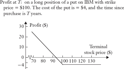
In practice, option investors are interested in their potential profits at all possible stock prices. For the above IBM option, Figure 19.1 plots the potential profits of the call at the option expiration date. Let's assume that the option price for the IBM call option is $5. The option buyer's profit is $5 (assume zero interest for simplicity) when the stock price ends up at S_T = $110 on the expiration day. The option buyer realizes $10 by exercising the call option. However, this amount must be reduced by the option price of $5, so the net profit from exercising the option is $5 = ($10 − $5). The profit is $15 when S_T = 120. However, if S_T ≤ 100, the buyer will not exercise the call and consequently incurs a maximum loss of $5, the purchase price. Figure 19.2 is a similar plot for the potential profits of the put option.

At any time t from today to expiration, an option holder can take one of three actions: (1) hold the option; (2) exercise (if the terms of the option permit early exercise); or (3) sell it. We say a call is:

out-of-the-money if the stock price is below the strike price, S_t < X

at-the-money if the stock price is equal to the strike price, S_t = X

in-the-money if the stock price is above the strike price, S_t > X

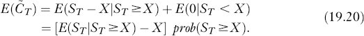
FIGURE 19.1 CALL VALUE AT EXPIRATION

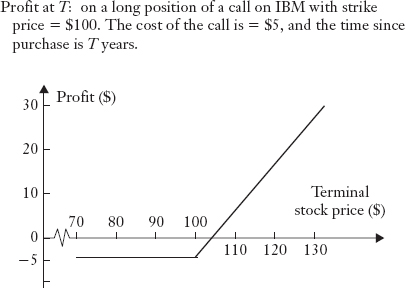
FIGURE 19.2 PUT VALUE AT EXPIRATION

For a put option, the same definitions follow, but with the inequalities reversed.

Clearly, the option buyer will only exercise an option when it is in-the-money. For example, for the IBM call option with a strike price of $100 (i.e., X = $100), the option buyer only exercises it when the stock price is above $100. This exercise value is known as the option's intrinsic value. In general, max(S_t − X, 0) is the intrinsic value for a call, and max(X − S_t,0) for a put. It should be noted that the intrinsic values are zero for out-of-the-money and at-the-money options.

Prior to expiration, the option buyer does not have to exercise the option when it is in-the-money. If the option buyer wants to realize the intrinsic value, all that need be done is to sell the option in market. Simple arbitrage assures that the option's price is at least as high as the value if it were to be exercised (i.e., the intrinsic value) and will usually be higher. The purpose of the option pricing theory discussed later in this chapter is to determine the fair price of an option.

19.2 SIMPLE USES OF OPTIONS

Why do we care about options? They are tools for both hedging and speculation. If an investor owns IBM stock, for example, and worries about the downside price risk for that stock, he can simply buy put options on IBM. For example, if the investor has one share of IBM stock with a price of $100 today and wants to avoid the risk of the price dropping to $80, he can buy a put with a strike price of $80. Then no matter how the stock price moves between the purchase date and the expiration date, the investor can always sell the stock for at least $80. In other words, with the put option, the floor value of the stock position is $80 over the life of the option. If he has a higher risk appetite, he can buy a put with strike price of $50. Buying a put is analogous to buying insurance, where the strike price is effectively the minimum price that will be received for an asset and the difference between the current price of the asset and the strike price is the deductible that the insurance buyer is willing to accept. Of course, the option price is the insurance premium (hence, the use of the term option premium as a synonym for the term option price). For example, suppose the stock price is $100 and the investor purchases a put option with a $70 strike price. The investor is willing to accept a loss of up to $30 if the price falls. Thus, the $30 is effectively the deductible. If, instead, the investor buys a put with a strike price of $80, he is only willing to accept a loss of $20 should the price fall and the deductible is $20. As with insurance, the greater the deductible the insurance buyer is willing to accept (i.e., the lower the strike price), the lower the cost of the insurance. In the case of a put, a put with a strike price of $70 (a deductible of $30) will cost less than a put with a strike price of $80 (a deductible of $20).

Consider now a speculative use for options. Suppose that IBM stock price is currently at $100, and a call with a strike price of $110 sells at $5 (i.e., option price). If an investor has $5,000, he can buy 1,000 options.² Then, if the stock price rises to $150 on the expiration day, each option will be worth $40 or a total of $40,000 for the 1,000 options. Hence, the return on the $5,000 invested in the call option position is 700% [=($40,000 − $5,000)/$5,000]. In contrast, if he had invested directly in the stock, the investor can buy 50 shares (= $5,000/$100), realizing a profit of $50 on each share or $2,500 on all 50 shares. The return in this case would be 50% [=($5,000 − $2,500)/$5,000].

While the investment in the call option generated a far superior return than investing directly in the stock, there is also a disadvantage of greatly increased risk. To see this, suppose that the stock price goes up to $105 rather than $150. The stock investment will generate a 5% return, but the option investment will suffer a 100% loss since all the call options will expire worthless. This simple example highlights the high risk and high return nature of option trading.

There are countless ways in which options can be used. For example, a popular bet is on news or earning announcements. Suppose that, prior to an announcement, it is unknown whether the news is good or bad. If one believes that a large stock price movement will follow the announcement, he can buy both a call and put on the stock, each with at-the-money (ATM) strike prices. In this way, whether the stock moves up or down, he can make money as long as the movement is sizable enough to cover the option price. This strategy is known as a straddle strategy, which is clearly difficult to do without the use of options. Moreover, since ATM options are more expensive than out-of-the money ones, the investor can buy the latter instead. Then the strategy is known as a strangle strategy.

19.3 PUT-CALL PARITY

The prices of a European call and a European put cannot be arbitrary. Rather, arbitrage possibilities mean they are related by the put-call parity relationship:

where D is the present value of dividends paid by the underlying stock over the life of the option, and PV(X) is the present value of the strike price. The intuition is that buying a stock and a put has upside potential and limited downside, as shown by the left-hand side of (19.3), and so is buying a call with risk-free investment of certain cash, as shown by the right-hand side of (19.3). Since both have the same payoffs in the future, in the absence of costless arbitraging³ their prices today must be the same. Note that although the formulation of put-call parity is in terms of options on individual stocks, the relationship holds for options on stock indexes and bonds. In the case of bonds, the dividends are replaced by coupon interest payments over the life of the option.

A rigorous proof of the put-call parity relation works as follows. Assume for simplicity that there are no dividends. Consider the payoffs of two portfolios. Portfolio A contains one share of the stock and a put. Portfolio B contains a call and an investment of the present value of X. Let S_T be the stock price at expiration. Then, as shown below, the two portfolios will always have the same payoffs on the expiration day regardless of the stock price:

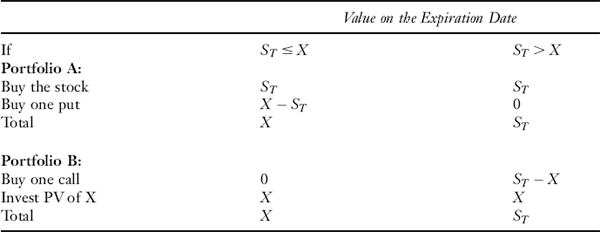
Therefore, the two portfolios must have the same price today if there is no arbitrage. This implies that the put-call parity must hold.

In option pricing, we usually use a continuously compounded interest rate. (See Web-Appendix J.) If today is time 0, and the time to expiration is T, then:

PV(X) = X_e^−rT

where r is the continuously compounded risk-free rate (annualized).

The application of put-call parity is straightforward. For example, suppose that a firm's stock sells at $50. Suppose that a put option, with strike price $45 and a maturity of 6 months is selling in the market at $3. Assume further that r = 5%. What price should a call option sell for?

Now we have:

S = $50, X = $45, P = $3, r = 5%, T = 0.5, D = 0

so the PV of the strike price is:

PV(X) = $45 × e^{−0.05 × 0.5} = $43.89

By put-call parity, we have:

C = S + P − PV(X) = $50 + $3 − $43.89 = $7.12

Note that the above put-call parity holds exactly for European options, but only approximately for American options. One reason is that either an American put or an American call may be exercised prior to maturity, while the other is still out-of-the-money.

19.4 KEY IDEA FOR VALUATION

The fundamental insights that lead to almost all option valuation formulae (i.e., formulae for determining the theoretical value of an option) are

• A suitable portfolio (called a replicating portfolio) of the stock and bond replicates the payoff of the option.
• A suitable portfolio (called a hedging portfolio) of the option and stock is risk free.

Then, if there is no arbitrage, the cost of the first portfolio (i.e., the replicating portfolio) must be the option price, and the return on the second portfolio (i.e., the hedging portfolio) must be the risk-free rate.

To obtain an option price, we have to make an assumption on how the stock price will move from today until the time when the option expires. Given such an assumption, we can obtain the theoretical option price based on either of the insights, used together with the assumption that there are no arbitrage opportunities.

19.5 SINGLE-PERIODB IN OMIAL MODEL

In this section, we provide a simple option valuation based on the key insights. To make the ideas and methods as easy to understand as possible, we assume a one-period and two-state model for the stock price. These assumptions will be relaxed later.

19.5.1 Replicating Portfolio

Suppose that a stock's price is $50 today, and that it can have one of two possible values next month: either $60 in the “up” state or $40 in the “down” state. Consider a European call option to buy the stock next month at the strike price of $55. If the monthly interest rate is r = 1%, what should the call price be?

Note that the call will be worth $5 if the stock is up, and $0 if the stock is down. Figure 19.3 illustrates the stock price tree and the payoffs to the option. Now we want to replicate the payoffs to the call. Consider a portfolio of 0.25 shares of the stock and the sale of a bond of $9.90. Selling the a bond is a means of obtaining funds (i.e., borrowing) to invest and is denoted by − $9.90. The construction of the portfolio consisting of the 0.25 shares of stock and the amount of bonds to be sold will be derived later.

FIGURE 19.3 REPLICATING PORTFOLIO

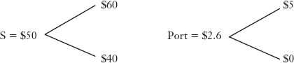
If the stock goes up to $60, the 0.25 shares of the stock will be worth $60 × 0.25 = $15. The sale of the bond means that not only must the $9.90 be repaid, but there is interest of $0.90 (1% interest for the month). So $10 must be paid to satisfy the bond obligation. Thus, the portfolio is worth the difference between the value of the shares ($15) and the bond repayment ($10) or $5. If, instead, the stock price goes down, the 0.25 shares of the stock is worth $10, which is just enough to pay the borrowing, so the portfolio is worth $0.

We have shown that the above portfolio replicates the payoff of the call. If there is no arbitrage, the cost of the portfolio must be equal to the cost of the call, implying that:

0.25 × $50 − $9.90 = $2.60

must be the call price.

The remaining question is: How do we construct the replicating portfolio? Suppose we need Δ shares of the stock and Bamount of bonds, then we want:

to replicate the payoff of the call. By solving the above two equations, we get Δ = 0.25 and. B = −$9.90.

The replicating portfolio says that, holding a call option is equivalent to the portfolio of holding Δ shares of the stock and a loan of amount B, that is,

In words, this says that:

That is, the call can be synthetically created by a portfolio of stocks and leverage such that the payoff of the portfolio replicates the payoff of the call, and this is why the portfolio is called the replicating portfolio (also referred to as the equivalent portfolio).

In general, if a stock with price S today will either go up to (1 + u)S or go down to (1 + d)S, where u > r and d < r, we solve

for the replicating portfolio, where C_u and C_d are the call values in the up and down states, respectively. The solution is easily obtained,

Equation (19.6) is the general formula for finding the composition of a replicating portfolio. Using equation (19.6) along with equation (19.4), we can write the call price as:

As will become clear later, the risk-neutral probability p can be interpreted as the probability from the perspective of a risk-neutral investor. Hence, the call price is simply the present value of its expected payoff, calculated under the risk-neutral probability. Equation (19.7) is a special case of the theory discussed in Chapter 16. Note also that the same formula is also applicable to a put option once the call payoffs are replaced by the put values. Alternatively, one can compute the put price by using the put-call parity.

Now, to value the previous call option, we can apply equation (19.7) directly without computing the replicating portfolio. We have u = 20%, d = 20%, and so:

p = (0.01 + 0.20)/(0.20 + 0.20)/0.525

Thus,

the same answer as before, as it should be.

19.5.2 Hedging Portfolio

Consider now the position of a market maker who sells a call to an investor and would like to buy Δ shares of the stock to hedge. That is, he has a portfolio consisting of (1) a short position in one call and (2) a long position in Δ shares of the stock. The value of this portfolio next month will be ($60 Δ − $5) if the stock goes up and $40Δ if the stock goes down.

How can the market maker arrange a risk free portfolio? If he buys Δ = 0.25 shares, then the value of the portfolio will be:

($60Δ − $5) = $40Δ = $10

regardless of which state is realized, that is, regardless of whether the stock goes up or down! Assuming as usual that there are no arbitrage opportunities in the economy, this portfolio must earn the same return as the risk-free rate. Since the cost of the portfolio is ($50 × 0.25 − C) = ($12.5 − C), where C is the call price and −C represents “negative” cost because the option market maker receives money from selling the call, we must have:

or C = $12.5 − $10/(1 + 1%) = $2.60.

Note that the replicating portfolio and the hedging portfolio are closely related. If SΔ + B replicates the payoff of a call C = SΔ + B, then SΔ − C must be the hedging portfolio because SΔ − C = B is risk free. The converse is also true. Hence, the number of shares Δ of the hedge portfolio (known as the hedge ratio), can be computed from equation (19.6) for hedging an arbitrary call.

19.5.3 Risk-Neutral Valuation

The replicating and hedging portfolio valuations provide profound insights into how option prices are determined. In particular, option prices have been shown to be independent of investors’ risk tolerance. Intuitively, no matter what level of risk tolerance an investor has, he will take any possible arbitrage opportunities because by definition such opportunities are riskless. Then, since the absence of arbitrage does not depend on investors’ risk tolerance, neither do option prices, which also rely on the absence of any possible arbitrage opportunities.

The fact that option prices do not depend on investors’ risk tolerance is of fundamental importance, leading to the so-called risk-neutral valuation. We can compute the option price in the real world (where investors have different levels of risk tolerance) by computing it in an imagined risk-neutral world where (1) all investors care only about the expected returns (not the risk as measured by standard deviations) and (2) the expected returns on all risky investments are the same as the risk-free rate.

Risk-neutral valuation is a simple method for computing option prices easily and quickly. Consider now how we apply it to compute the earlier call price of $2.6. In a risk-neutral world, the expected return on the stock must be the risk-free rate of 1% per month, so:

p$60 + (1 − p)$40 = $50(1 + 1%)

where p is the risk-neutral probability that the stock to go up, and (1 − p) is the risk-neutral probability for the stock to go down. Solving the above equation, we have:

p = 0.525

Now, using this probability, we can compute the expected payoff on the call option,

0.525 × $5 + (1 − 0.525) × $0 = $2.625

Since the option should produce the risk-free return in a risk-neutral world, its present value discounted by r should be its price today, that is,

In general, if a stock price either goes up to (1 + u)S or goes down to (1 + d)S, the risk-neutral probability must satisfy:

p × (1 + u)S + (1 − p)×(1 + d)S = S×(1 + r)

Then:

The expected payoff on a call option is then:

pC_u + (1 − p)C_d

and so the call price is the discounted expected payoff,

This is the same formula as equation (19.7). Note that the risk-neutral probability is a function of the stock growth rates (i.e., the amount by which the stock can go up or down) and r, but does not depend on any call or put features.

For a further clarification, consider another example. A firm's stock sells at $100. It is known that the price will be either $125 or $75 a year from now. Thus, u is 0.25 and d is −0.25. Assume that the annual risk-free interest rate is 4%. What price should a European call option with a strike price of $110 and a maturity of one year sell for? One can solve the problem in three steps. First, find the risk-neutral probability,

p = (r − d)/(u − d)/(0.04 + 0.25)/(0.25 + 0.25) = 0.58

Second, find the expected payoff of the option at the time of its expiry,

p×$15 + (1 − p) × $0 = $8.70

Third, get the time 0 option price by discounting the expected payoff,

C = $8.7/(1 + 0.04) = $8.37

19.6 BLACK-SCHOLES FORMULA

In this section, we provide the famous Black-Scholes option valuation formula. We first lay out the key assumption that the stock price follows a lognormal distribution, then compute the option price based on the no-arbitrage principle. Finally, we discuss various features of the formula.

19.6.1 Log normal Stock Price

We have so far computed option prices by assuming stock prices can change according to two states of the world, clearly a simplistic assumption. Another model for describing the movement in stock prices is a random walk, in which a stock price is assumed to evolve according to:

where ∊_t+1 is a noise term. This model says that tomorrow's stock price is today's price plus a random noise. The noise ∊_t+1 is a normal random variable with zero mean and standard deviation σ. The standard deviation σ reflects the magnitude of fluctuations in the price. For example, assume today's price is S₀ = $50 and the standard deviation of ∊_t+1 is 2. Some good and bad news may successively shock the stock price by, say, ∊₁ = 0.85, ∊₂ = −1.34, ∊3 = 0.28, and so on. Then the price will be S₁ = 50 + 0.85 = $50.85, S₂ = 50.85 1.34 = $49.51, S₃ = 49.51 + 0.28 = $49.79, and so on.

To understand better the random walk model, it will be useful to review two definitions of the rate of return before proceeding further. The first definition is the discrete return or simple return given by:

the percentage change in price. The second is the continuously compounded return, given by:

the rate of change in price expressed as a natural logarithm. If today's price of $50, and if the future price is either $25 and 0, then the simple returns are −50% or −100%. A simple return of200% does notmake any sense, since the simple return is both bounded from below and asymmetric. On the other hand, the continuously compounded return is well defined for any value. For example, the continuously compounded returns of 50%, −100%, and −200% mean the future stock price is $33.33 (= 50e^−0.5−1), $18.40, and $6.77, respectively. In pricing derivatives, continuously compounded returns are used instead of simple returns to be consistent with the assumption that prices move continuously over continuous time. The continuously compounded return is often assumed to be normally distributed, further implying that it is symmetric around 0. In addition, the volatility used in derivatives is the standard deviation of the continuously compounded return, not that of the simple return.

Going back to the the random walk model given by equation (19.10), despite its popularity, there are two problems. The first is that the normal random variable has a positive probability of realizing a large negative number. For instance, in the earlier example with S0 = $50, ∊₁ can be less than −$50 with positive probability, and then S₁ < 0. This is clearly not possible in the real world. A simple way to resolve the negative stock price problem is to assume that the logarithm (log) of the price is a random walk. That is,

In this case, the future price S_t+1 = S_te^∊t+1 will always be positive if today's price is positive.

The second problem with the random walk model is that the expected return of the stock is zero, which is also unrealistic. Suppose μ is the annual expected return. We can add it into the above equation (19.13) to obtain:

where N(0, σ²)denotes the normal distribution with mean zero and variance σ².

The last two changes lead us to the next fundamental assumption underlying the famous Black-Scholes formula:

Assumption 1: The continuously compounded stock returns, ln(S_t+1/S_t), are independent over time, and identically normally distributed with mean μ and variance σ².

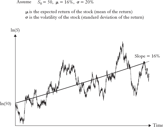
This assumption is also known as the geometric random walk model, geometric Brownian motion, and lognormal stock price model. Figure 19.4 is helpful in understanding the assumption. Assume that the stock price is $50 today, and its average growth rate or expected return is μ = 16%, with 20% annual size of fluctuations (i.e., annual volatility). In the absence of risks, the stock should grow at 16%, that is, its prices over time should be the straight line with slope 16%. However, as good and bad news is released along the way, the actual price path is the up and down curve, with the size of annual fluctuation being normally distributed with an annual volatility of 20%.

FIGURE 19.4 PRICE UNDER LOGNORMAL ASSUMPTION

The lognormal assumption is additive in that the sum of two lognormal returns remains lognormal. Suppose today is time 0. Over T periods, the total return is:

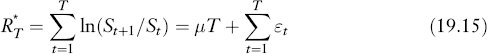
The expected return and variance are:

This says that the expected return grows linearly with time T, but the standard deviation (known also as volatility) grows at . Since R_T* = ln(S_t+1/S_t), we can also write the lognormal assumption as:

ln(S_T) ~ N[ln(S₀) + μT, σ² T]

Taking exponential on the both sides, we have the assumption in terms of price,

where is a standard normal random variable with mean zero and variance 1. This equation will be useful later.

19.6.2 The Formula

Recall that in our one-period two-states model, a call option price is given by:

i.e., the price takes the form of an expected payoff discounted at the riskless rate. This is also the risk-neutral valuation principle discussed in Chapter 16. Hence, even under the lognormal assumption, we still have:

where r is the continuously compounded risk-free rate (usually annualized) and T is the time (from today) to maturity of the option (usually measured in years). The key now is to compute the expected payoff, E(), under the lognormal assumption.

Since =(S_T − X,0)⁺, we can decompose E() into two terms,

By transforming ln S_T into the standard normal random variable, we can then compute the two terms explicitly (see the appendix to this chapter), and hence, obtain the most useful and famous Black-Scholes formula for option pricing for the price of a European call,

where

and

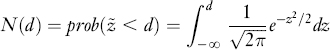
is the cumulative normal distribution function, that is, the probability that a standard normal random variable is less than a given number d. In practice, N(d) can be easily computed by using the Excel function normsdist. For example, N(0) = normsdist (0) = 0.5, N(1) = normsdist(1) = 0.8413, etc.

The Black-Scholes formula given by equation (19.21) provides a price of a European call option on a non-dividend-paying stock (the dividend case will be discussed later). To compute the call price, there are five parameters to supply:

1. S = current stock price
2. X = exercise or strike price
3. r = risk-free rate (continuously compounded) over the life of the option
4. σ = standard deviation (volatility) of (continuously compounded) stock returns
5. T = time to expiration date or maturity

Note that S, X, and Tare directly observable, but r and σ are not. They have to be estimated, which will be discussed later.

Consider now how to implement the Black-Scholes formula. Assume a stock that pays no dividends for the next three months is selling at $30. The annual risk-free rate is estimated to be 6% and volatility is estimated to be 50%. We ask two questions. First, what is the price of a call with strike $35 and time to expiration three months? Second, what is the price of a put option with the same strike and time to expiration?

Here we have

S = $30, X = $35, T = 3 months, σ = 0.5, r = 0.06

Since r is here assumed to be the continuously compounded annual interest rate, T should also be in annual form; that is, T = 3/12 = 0.25 years.

To obtain the price of the call, we compute first d₁ and d₁:

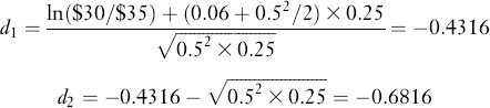
Then, by using Excel or a relevant software package, we get the values of the cumulative normal distribution function,

Then, plugging these into the Black-Scholes formula given by equation (19.21), we have:

Given the price of the call, we now use put-call parity to get the price of the put as follows:

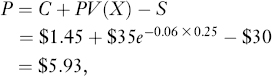
where we have computed the present value of the strike price using continuous discounting, because r is the continuously compounded interest rate.

How do we interpret the terms in the Black-Scholes formula? The same replicating portfolio interpretation,

holds in both the previous binomial model and in the lognormal model here. It is just that the two models imply different forms of Δ and B. Now we have Δ = N(d₁), which is the delta or hedge or the number of shares one needs to buy today to replicate the payoff of the call. This is also roughly the amount of money the buyer of the call makes when S goes up by $1. In the example here, the call seller should purchase N(d₁) = 0.333 shares of the stock to hedge the call.

The term Xe^−rT N(d2) is the analogue to Bin equation (19.22), the amount of money one borrows to finance the purchase of the stock in the replicating portfolio. Note that both d₁ and d₂ are transformations to link the log stock price to the standard normal random variable, and they have no obvious economic interpretations.

In addition, based on the proof in the appendix to this chapter, N(d₂) is the risk-neutral probability for the option to make money. It is 24.77% in the previous example. However, it should be pointed out that this is different from the true probability, N(d*₂), where:

is a function of μ, the expected continuously compounded return on the stock. The expected return is μ = r − σ²/2 if the risk-neutral probability is the same as the true probability. The derivation of N(d*₂) is the same as N(d₂), except now the objective probability is used. In the earlier example, if μ = 15%, then d*₂ = 0.4666 and N(d*₂) = 33.3%. Intuitively, the objective probability is what risk-averse investors believe the stock will exceed the strike price, and in a risk-averse world it must be higher than the risk-neutral probability.

The Black-Scholes formula is the first model recognizing that options are replicable assets and can be priced given the underlying asset price and other parameters. It provides profound insights for subsequent derivatives theory and practice.⁴

19.6.3 Accounting for Dividends

The Black-Scholes formula assumes no dividends. But stocks do pay dividends in practice. It is clear, however, that only those dividends over the life of the option will matter in the option price. We consider two types of dividends here. The first is discrete where the dividends are paid over a finite number of dates prior to maturity. This is the case for individual stocks in practice. The second is continuous dividends where the dividends can be viewed as being paid continuously, such as holding a stock index or a foreign currency (the foreign interest rate plays the role of dividends).

For European options, dividends can be accommodated straightforwardly. We can simply apply the Black-Scholes formula to the dividend-adjusted price, that is, the stock price excluding the present value of the dividends. The reason is that when the dividends are fully anticipated, the stock price will drop each time by the amount of dividends that are paid out. One can imagine that there are two identical firms. One pays out all the dividends today by its present value and another pays out sequentially. Since both firms pay out the same present value of dividends, their values must be identical on the option expiration day, which is what matters for the European option holder. Hence, the option on the second firm must be identical to that on the first, but the second has no dividends over the life of the option.

If dividends are discrete and paid according to a known series, {D₁, D₂,…, D_m}, to be paid at 0 < t₁, t₂,…, t_m≤T, then the dividend-adjusted stock price is

The option price is then:

where

For example, suppose that S = $50, X = $50, T = 0.25, σ = 50%, r = 6% and the stock pays $2 dividend in one month, that is, D₁ = 2 with t₁ = 1/12. Then S_D = S − D₁e^{−0.06 × 1/12} = $48.01. Applying the Black-Scholes formula given by equation (19.21) for S_D, the call price is $4.24. A put price is computed similarly. For example, the put price with the same strike is

P = C − S_D + PV(X) = $4.24 − $48.01 + $50e^{−0.06 − 3/12} = $5.49

Note that the put-call parity relation applied here is the one without dividends, because S_D has already adjusted for the dividends. One can also apply the version with dividends, but then S has to to used. The answer will obviously be the same.

For European options with continuous dividends, the present value of the dividends is:

where δ is the annual dividend yield rate. Then, the dividend-adjusted price is:

Plugging this into the Black-Scholes formula and rearranging terms, we obtain:

where

For the price of a European put a similar formula,

holds.

19.6.4 Estimating r

The Black-Scholes formula is a function of five parameters, S, X, r, σ, and T (and a sixth, δ if there are dividends), of which the risk-free rate rand volatility σ have to be estimated in practice. It is easy to estimate r from financial market data. For short-term (less than 1 year) options, a proxy for r may be chosen as the continuously compounded annual rate of return for holding a U.S. Treasury bill. For example, suppose that the face value of a 90-day Treasury bill is $100 and the cash price is $99.30. Then r is obtained by solving $100 = $99.30e^r×90/365, that is, r = 2.85%. For long-term options, r is extracted from Treasury note prices.

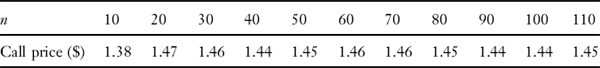
Theoretically, r is the rate of U.S. Treasury security whose maturity matches the remaining life of the option. So, for short-term options, the maturity of the Treasury bill should be close to the maturity of the option. This, however, seldom matters because the option price is fairly insensitive to the risk-free rate. To see this, consider our earlier example with S = $30, X = $35, T = 0.25, σ = 0.5, r = 0.06, d = 0.0, the call price is $1.45. Allowing the risk-free rate to go up from 1% to 10%, we have:

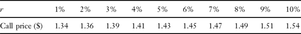
The above results show how the call price varies with the risk-free rate. Small differences or estimation errors in r do not make a substantial difference in the option price.

19.6.5 Estimating σ

In contrast, the call price is very sensitive to the value of volatility. In the above example, if we allow σ to vary, we have:

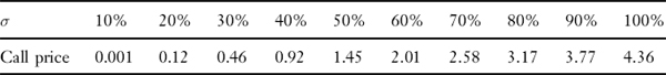
We see from the above the call price varies from virtually worthless to $1.45at the true volatility of 50%. For the same percentage of estimation error in σ, it has a much greater impact on the option price than the error in r. It is, hence, very important to estimate the volatility accurately in practice.

In the Black-Scholes formula, the volatility is the standard deviation of the continuously compounded stock returns over the life of the option. It is both one of the most important factors in determining an option price, and one of the most difficult to estimate. This is because no one knows what future volatility will be for the remaining life of the option. Nevertheless, there are two widely used methods for its estimation. The first is to use historical stock prices and obtain the so-called historical volatility. The second is to use an observed option price to back out a volatility at which the Black-Scholes formula price is equal to the observed option price. This volatility is implied by the option price, and so it is called the implied volatility.

19.6.5.1 Estimating Historical Volatility

The computation of the historical volatility can be carried out in four steps:

Step 1: Decide whether to use daily, weekly, or monthly prices, and how many of them.

Step 2: Compute the continuously compounded returns as follows

where S₀, S₁, S₂,…, S_n are the stock prices, and D_ivi is zero or the amount of the dividends at i if there are any.

Step 3: Use Excel or other computer software to obtain the standard deviation of R*_i, say s.

Step 4: Transform the historical volatility s into annual form,

where τ is the number of the intervals of the data in a year. For example, for daily, weekly, and monthly data, respectively. However, investors usually adjust the daily volatility by the number of trading days rather than by the number of the calendar days. Following this convention, should be used for daily data. For example, if the estimated daily standard deviation is 1%, then . Since all parameters of the Black-Scholes formulas are usually measured in annual form, it is important to remember to annualize the standard deviation.

19.6.5.2 Estimating Implied Volatility

Consider now how to compute the implied volatility. This is best understood by using an example. On one day, Microsoft's stock price was , and the call option with strike $85 sold at . With the following additional information,

S = $80.375, X = $85, T = 0.1945, r = 2.79%, d = 0.0

we are ready to compute the call price by using the Black-Scholes formula for any given value of σ. Although now we know C=$2:875, σ is unknown and needs to be backed out.

To find σ, we can start from a low value of σ and a high value of σ. A value of σ = 10% roughly says that the stock return is likely to be 10% up or down from the coming year, and is probably a low estimate for the volatility of most stocks. On the other hand, σ = 100% is a high estimate. Computing the call price at σ =10%, denoted as C(σ = 0.10), and doing the same for σ = 100%, we have:

C(σ = 0.10) = $0.2278, C(σ = 1.00) = $12.4018

Note that the observed price C = $2.875 is between C(σ = 0.10) and C(σ = 1.00), the volatility has to be between 0.10 and 1.00 because the call price is an increasing function of the volatility.

Now computing the call price at the middle point between 0.10 and 1.00, we have:

C(σ = 0.55) = $6.0472

Because the observed price C = $2.875 is between C(σ = 0.10) and C(σ = 0.55), the volatility has to be between 0.10 and 0.55. Computing the call price at the middle point between 0.10 and 0.55, we have:

C(σ = 0.325) = $2.9168

Because the observed price C = $2.875 is between C(σ = 0.10) and C(σ = 0.325), the volatility has to be between 0.10 and 0.325. Computing the call price at the middle point between 0.10 and 0.325, we have:

C(σ = 0.2125) = $1.4361

Because the observed price C = $2.875 is between C(σ = 0.2125) and C(σ = 0.325), the volatility has to be between 0.2125 and 0.325.

Proceeding in the process as above, we will find that:

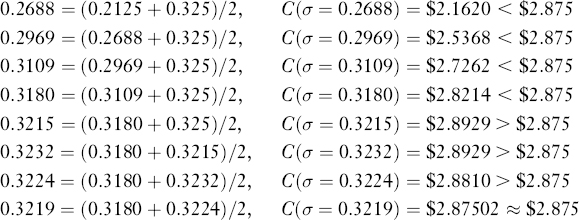
So, the implied volatility is σ = 0.3219 = 32.19%. It is easy to program the above procedure, referred to as the bisection method, into a computer to find the implied volatility quickly.

A more efficient (but less intuitive) procedure is the Newton-Raphson algorithm. The algorithm finds the root of a function; that is, a solution to f(x) = 0, successively by iterating from any initial value x₀ via:

x_i+1 = x_i − f(x_i)/f′(x_i)

where i = 0, 1, 2, 3,…, till convergence. Since now the implied volatility is the solution to C(σ) − $2.875 = 0, we compute:

based on an arbitrary starting value, say, σ0 = 1.0. Then, σ1 = 0.3225, σ2 = 0.32192, and σ₃ = 0.32192. The algorithm finds the answer in two steps.

While traders may come up with different estimates of the historical volatility, their estimates of the implied volatility should be the same if they agree with the Black-Scholes formula. The implied volatility represents the current market's assessment of the volatility of the underlying security, whether it is a stock, a commodity, or a stock index. This is useful not only for option traders, but also to stock investors for estimating the current riskiness of the market.

With the use of implied volatility, the price given by the Black-Scholes model is matched to the option's market price. A question is why we compute the volatility by using the option price, and not the other way around as we usually do. The answer is that the option market contains the information about the stock volatility of all traders, and this is reflected in the traded option price. Based on one such option price that provides the current assessment of volatility, the Black-Scholes formula can then help to price all other options, with different strikes and maturities, on the same stock and options on assets closely related to the stock.

19.6.6 Measuring Price Sensitivity to Inputs: The Greeks

As we have seen, the following factors determine the option's price: (1) current stock price, (2) strike price, (3) interest rate, (4) volatility in the stock price, (5) time to expiration, and (6) cost of carry (dividends for stocks). Given these factors, we can use the Black-Scholes formula to compute the price of any European option. This section investigates how changes in these factors will affect the option price.

Consider how the stock price affects a call based on the Black-Scholes formula with continuous dividends. The intuition is that a call option allows one to obtain a stock in the future for a fixed price (strike price). Other things being equal, the higher the stock price, the more valuable the call option and, therefore, the higher should the call price be. Mathematically, the partial derivative of the call with respect to the stock price, known as the option's delta, is:

where the right-hand side is the partial derivative of the Black-Scholes call price, equation (19.28), taken with respect to the stock price. The Δ is also the hedge ratio that measures the changes in a call price due to the changes in a stock price.

The option's gamma, denoted by Γ, measures the rate of change in the option's delta with respect to change in the stock price,

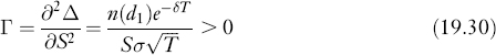
where . This says that the delta increases as the stock price goes up. If Γ is small, delta changes slowly with respect to S. If Γ is large, the delta is more sensitive to changes in S.

The call price is clearly a decreasing function of the strike price,

Intuitively, the higher the payment for exercising a call option (i.e., the higher the strike price), the less valuable the option.

The effect of the changes in the interest rate, referred to the option's rho and denoted by ρ, is:

This says that the value of a call is positively related to the level of interest rates. Intuitively, the higher the interest rate, the lower the present value of the payment for exercising the option to buy a stock whose value remains the same, and so the more valuable the option.

Volatility is the key factor determining the option price. The change in the option price with respect to the change in volatility is referred to as an option's vega and is usually denoted by:

This states the well-known fact that the call price rises as the volatility goes up. The Vega of a put is also positive. Intuitively, a stock may go up or down. A call or put allows one to obtain either the upside or downside potential while risking only the premium (the money paid for the call or put before the change in the volatility takes place). The greater the volatility, the greater the upside or downside movement. Thus, a larger volatility allows a greater potential payoff. Hence, the call or put must be more valuable if the volatility rises.

The impact of the changes in time to expiration is called the option's theta, denoted by Θ, and is measured by:

and can be either positive or negative. Intuitively, the longer an option's life, the higher the stock price may grow, and so the more valuable the option. On the other hand, the stock price may not grow at all if it pays too much in dividends. However, the dividends for stocks are usually small, and when this is the case, theta is unambiguously positive. Indeed, in practice, it is almost always the case that the longer the life of the option, the more valuable the option.

TABLE 19.1 IMPACT OF PARAMETERS ON OPTION VALUE

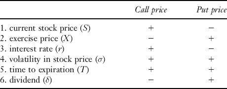
Finally, the impact of dividend changes is measured by

This says that the relationship between the call price and the cost of carry is positive. Intuitively, the higher the dividend, the more money goes to the shareholders, and hence, the less valuable the call option.

All the above partial derivatives, which measure how the option price will change as one of the six parameters varies, are known as Greeks.⁵ The qualitative relationships are summarized in Table 19.1.

19.7 BINOMIAL MODEL

In this section, we extend the earlier one-period binomial model to multiple periods. The model complements the Black-Scholes formula. It not only converges to the Black-Scholes price for European options, but is also applicable to American options.

19.7.1 Multiple Periods

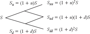
The one-period binomial model allows only two possible values of the stock price at the expiration date, assumed here to be one month. As already noted, this is an unrealistic assumption, and we would like to increase the number of possible values. To get three possible values, we can extend the one-period model to a two-period model by assuming that the stock with price S will either go up to (1 + u)S or go down to (1 + d)S in the first half of the month; (1) if it goes up to (1 + u)S, it may go up again to (1 + u)](1 + u)S] = (1 + u)²S or go down to (1 + d)[(1 + u)S] = (1 + d)(1 + u)S in the second half of the month; (2) if it goes down to (1 + d)S, it may go up to (1 + u)[(1 + d)S] = 1 + d)(1 + u)S or go down again to (1 + d)[(1 + d)S] = (1 + d)²S in the second half. Thus, at the end of the month we have three possible values of the stock price:

(1 + u)²S, (1 + d)(1 + u)S, (1 + d)²S

This is illustrated in Figure 19.5.

FIGURE 19.5 A TWO-PERIOD BINOMIAL MODEL

The question is how do we price a call option now. The idea of recursive discounting is widely used in practice for the valuation of complex derivatives. We can apply the one-period model recursively to discount the payoffs back period by period till today. The call prices in the half month when the stock is up or down are:

where p = (r − d)/(u − d) and C_ud = C_du. Thus, the call price today is the discounted expected payoff:

Mathematically, one can verify that the replicating portfolio costs exactly C today. Although the portfolio will adjust next period, no future inflow or outflow of capital is needed since on the expiration date, its payoffs will equal the option payoffs in all three states of the world.

For example, consider a stock selling at $50 that will either go up at the rate of u = 25% or go down at the rate of d = −25% in each month for the next two months. Assume the constant risk-free rate is 1% per period. Then from equation (19.37) the risk-neutral probability is p = (0.01 + 0.25)/(0.25 + 0.25) = 0.52. For a call with a strike of $55, its payoff (1) when the stock price is up next period is C_u = (p×23.125 + (1 − p)×0)/1.01 = $11:91, and (2) when the stock price is down is C_d = $0. Hence, the price today must be C = (p×11.91 + (1 − p)×0)/1.01 = $6.13. For a put option with the same strike price, we can either compute its value the same way by replacing the payoffs of calls in each node of the tree by those of the put or by using the put-call parity. In the latter case,

P = C − S + D + PV(X) = $6.13 − $50 + $0 + $55/(1 + r)² = $10.05

where (1 + r)² is used to compute the present value of the strike price because there are now two periods to expiration.

The two-period binomial model allows three terminal values of the stock price. To allow four possible values, we need a three-period binomial model. In this case, the terminal values in the third period are:

(1 + u)³(1 + d)⁰S, (1 + u)²(1 + d)¹S, (1 + u)¹(1 + d)²S, (1 + u)⁰(1 + d)³S

In general, we can model the movement of a stock price to have (n+1) values in the n-th period by using the n-period binomial model. The terminal values are:

To obtain the call price in this case, similar to the 2-period binomial model, we can work backward from the tree and obtain the call price.

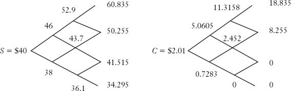
For example, consider a stock selling at $40 that will either go up at the rate of u = 15% or go down at the rate of d = −5% each month for the next three months. Assume the constant risk-free rate is 1% per month. In a 3-period model, for the price of a call option with a strike $42 and three months to maturity, we compute first the stock price tree forward, and then the option price tree backward. The results are shown in Figure 19.6. For instance,

C_uu = (0.3×$18.835 + (1 −0.3)××$8.255)/(1 + r) = $11.316

and

C = (0.3×$5.061 + (1 −0.3)×$0.728)/(1 + r) = $2.01

FIGURE 19.6 ATHREE-PERIOD CALL VALUATION

19.7.2 Relation to Black-Scholes Formula

Given S, X, r, σ, and T, we can compute the price of a European call option on a non-dividend-paying stock by using the Black-Scholes formula. Alternatively, we can compute the price by using the binomial model. The question is how the two prices are related to each other.

To match the lognormal assumption of the Black-Scholes formula, we choose:

in an n-period binomial model with ΔT as the per period time.⁶ Then, the larger the n (the greater the number of periods we use in the binomial model), the closer the binomial tree to the lognormal price, and so the closer the binomial price to the Black-Scholes price. In the limit, they are equal.

For example, consider the earlier call with:

S = $30, X = $35, T = 0.25, σ = 0.5, r = 0.06, d = 0.0

The Black-Scholes price is $1.45. Now, with using the n-period binomial model, we obtain the call price:

Theoretically, the price converges to $1.45 with an error of order 1/n, but the error oscillates, that is, it does not decrease monotonically with n.

Analytically, note that if the terminal stock price does not go up enough, the value of the call, max[(1 + u)^n−j (1 + d)^jS − X,0], is zero. Let a be the smallest nonnegative integer such that a ≥ ln[(1 + u)ⁿS/X]/ln[(1 + u)/(1 + d), then max[(1 + u)^n−j(1 + d)^jS − X,0] = 0 when j ≥ a and S − X when j, < a. So, we can compute the call price as:

where r* = e^rΔT − 1,

By the central limit theorem of probability theory, one can show that Φ(n)→N(d₁) and Ψ(n)→N(d₂) as n → ∞. That is, the binomial price converges to the Black-Scholes price with the parameter choice as given by equation (19.38).

19.7.3 Accommodating Dividends

The binomial model is far more flexible than the Black-Scholes formula. It can both deliver the Black-Scholes formula result, and also be easily generalized to compute options on assets that pay either discrete or continuous dividends. For discrete dividends, one can build the binomial tree with enough periods so that the dividends are paid at the end of periods in the tree. Then, one can compute the option prices the usual way by using the ex-dividend stock prices.

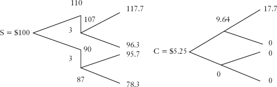
For example, assume that a stock with price $100 will either go up at u=10% or go down at d = −10% for the next two months. The stock will pay a $3 dividend next month and r = 1%. Let's demonstrate how to price a call with strike X = 100 and maturity of two months. We first compute the stock price tree forward. The price next month will be either $100 or $90. The only difference from before is that now the price will grow from its ex-dividend price, $107 or $87 to the second month. The final stock price is on the left-hand side of Figure 19.7. Computing the call payoffs at expiration as usual by taking the differences between the stock prices and the strike, we obtain those values on the right-hand side of Figure 19.7. Discounting them back period by period as before, we get the call price today as $5.25.

For continuous dividends, one can build the binomial tree the same way as before. However, the risk-neutral probability needs be adjusted as follows:

This adjustment is needed because, under the risk-neutral probability, the stock price appreciation combined with the dividends should earn the risk-free rate, and so the price should grow at a rate of (r−δ)ΔT per period, that is,

FIGURE 19.7 A CALL ON A DIVIDEND-PAYING STOCK

The solution to this equation leads to equation (19.39), which reduces to equation (19.38) when δ = 0. Then the valuation will be the same as the case when there are no dividends.

19.8 AMERICAN OPTIONS

For ease of study, our discussion so far focused on European options. Many real-world options, such as options on the S&P 500, are indeed European options where the option holder can only exercise the option on the expiration day. However, individual stock options, options on the S&P 100 (the most actively traded index option), and many others are American type where the option holder can exercise the option any time up to and including the expiration day. By incorporating the early exercise feature into our previous analysis, we can come up with the value of American options.

First, we note that the value of an American option should be at least as large as that of the corresponding European option on the same terms. This is because the American option has all the privileges of the European option and the additional privilege of early exercise. Using lowercase letters for European option prices and uppercase letters for American option prices with the same terms, we have:

C = c + ∊_C

P = p + ∊_P

where ∊_C and ∊_P are both nonnegative quantities called early exercise premiums.

For American calls on non-dividend-paying stocks, a somewhat surprising result is that it will never be optimal to exercise early and so the early exercise premium is zero. That is, the American call and European call have the same value in the zero dividend case. To see this, assume an American on a stock with strike $45 is available. The stock price is S = $50. Consider (a) a portfolio consisting of the call and $45 cash, and (b) a portfolio consisting of the stock. On the expiration day, portfolio (a) will have the value of at least the stock plus interest income from investing the $45 of cash and so the cost of portfolio (a) must be higher than that of portfolio (b); that is, C + $45 > $50 or C > $5. By exercising the call, only $5 is realized. So the option holder should not exercise the call. If the option holder needs the money or thinks the stock is going to drop, he should sell the call for C > 5 in the option market.

However, there always exists the possibility of early exercise for American puts even on non-dividend-paying stocks, implying that American puts are never worth less than European puts. For example, suppose a put with strike $100 was purchased awhile ago when the stock price was $120. It is always possible for the price to drop dramatically to S = $1 today. Assume the option still has a year to maturity. If the option holder waits to the expiration day, the maximize value is $100. But if the option holders exercises the option today, $99 can be realized which, in turn, can be invested at the risk-free rate, say 3%. Consequently, by exercising the option holder will get more than $100 next year. Hence, the option holder will exercise the option early and this is always possible.

As mentioned earlier, the binomial model is flexible and can be easily adapted to compute the price of American options. In contrast with European options, the key here is that on any node of the tree, the value of an American option is the maximum of its discounted expected payoff or its exercise value. The same holds for the put. That is,

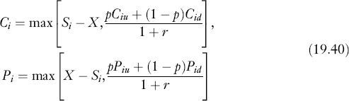
To see why, notice that the option holder can either wait or exercise the option at the node. If the option holder waits, he gets the discounted expected payoff. If he exercises, he gets the exercise value. The option holder will select the course of action that provides the higher value.

For example, in Figure 19.7, if the call is now an American style one, and if we exercise in the first month when the stock price is up, we exercise prior to the dividend payout to get $10 (=$110 − $100). If we wait, the wait value is the European value of $9.64 =(p×$17.7 +(1 − 0.55)×$0)/(1 + 0.01), which is lower. Hence, the American value at the node should be $10 rather than $9.64. Discounting back, we obtain the American call price as $5.45, which is $0.20 greater than the European call.

19.9 ARBITRARY PAYOFFS AND GENERAL MODELS

While our analysis has been focused on standard option payoffs, the risk-neutral valuation method is straightforwardly applied to compute any European type option with an arbitrary payoff function VT = V(S_T), where V(·) is a function of the terminal stock price. In a binomial tree model, we simply discounted the payoffs of V_T successively back to today. In the lognormal model, we compute now the discounted expected payoff under the risk-neutralized lognormal distribution,

where V₀ is the value today at time 0 of the derivative, and the tilde sign, as usual, emphasizes that the payoff is random. This equation is the same as before, that is, we replace in equation (19.19) by . However, we cannot derive a simple expression like the Black-Scholes formula for a general function V(·).

Numerically, one can easily compute V₀ via Monte Carlo simulation.⁷ The key is to compute the expected payoff of the derivative. Since equation (19.41) uses the risk-neutralized expected payoff, we must also use the risk-neutral distribution of the stock price rather than the true or objective distribution. To do so, we can simply use equation (19.17) with the risk-neutralized mean μ = r − σ²/2. By using simulation software, we can simulate a normal random variable , and then can use equation (19.17) to compute a random terminal stock price. We can do this thousands of times to get thousands of prices. The average of the discounted payoffs over all of these prices will be a good approximation to V₀. The approximation error is random, but its standard error converges to zero at a rate inversely related to the square-root of the number of simulated prices.

The payoff function V(·) can also depend on the path of the asset price. In addition, the asset price can be allowed to move over time with jumps, and the volatility can also be allowed to change stochastically. The above methods can be adapted to accommodate all these extensions.⁸

Appendix 19.1 Derivation of the Black-Scholes Formula

In this appendix, we derive the Black-Scholes formula. Note first that the risk-neutral valuation is generally valid, as shown for the single-period binomial model in Section 19.8 and for the finite states model in Chapter 16. For the lognormal or Brownian motion prices, a rigorous proof requires stochastic calculus.⁹

Given the risk-neutral valuation method, we need to find the distribution of the stock price under the risk-neutral probability. Since:

We have, from equation (19.17), that:

Under the risk-neutral probability, the expected return should be the risk-free rate, and hence, μ = r − σ²/2 or .

To derive the Black-Scholes formula, we need only to compute the two expected values in equation (19.20). Denote by f(S_T) the lognormal density function of S_T. Then:

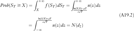
where μ = r − σ²/2. The first step follows from the definition for computing the probability, the second makes a transformation of variable,

the third reverses the direction of the integral, and the final step follows from the definition of N(d₂). In addition,

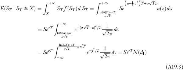
where the steps are similar to the previous one.

KEYPOINTS

• In contrast to futures and forward contracts, which have a linear payoff function, option payoffs are nonlinear functions of the underlying asset price. The fundamental valuation principle of option valuation is the absence of arbitrage opportunities.
• The fundamental insight is that option payoffs can be replicated by suitable positions in the underlying asset and the risk-free asset. Hence, the option price must be equal to the cost of the replicating portfolio.
• The hedging portfolio is a risk-free portfolio consisting of a short position in an option and a suitable holding of the underlying asset. It is closely related to the replicating portfolio.
• The price of a European call option is tied to the price of a European put with same underlying, strike price, and expiration date by a relationship called put-call partity. This relationship is only approximately true for American options.
• Risk-neutral valuation is used to compute the option price as its discounted expected payoff with the risk-free rate as the discount rate, while the payoff is adjusted for risk by using the risk-neutral probability.
• In a binomial model of the stock price, the option price can be computed backwards successively by discounting the expected future payoffs period by period.
• In a lognormal model of the stock price, the option price for a European call can be computed by using the Black-Scholes formula, and the European put price can then be computed using put-call parity.
• For European options on a dividend-paying stock, the Black-Scholes formula can still be employed by applying it to the dividend-adjusted price, which is the current stock price less the present value of the expected dividends.
• The volatility used in the Black-Scholes formula is the standard deviation of the continuously compounded stock return over the life of the option. It is the most important parameter that determines an option price, and can be estimated by either using historical volatility or implied volatility.
• With compatible choice of parameters in the binomial model, the binomial price converges to the Black-Scholes price as the number of periods approaches infinity.
• An American option on a non-dividend-paying stock will not be optimally exercised prior to expiration, and hence, its price will be identical to the corresponding European call. However, for a dividend-paying stock, the American call price will in general be greater than the corresponding European call price.
• An American put option has a positive probability of being exercised regardless if dividends are expected, and hence, its price is always greater than that of the corresponding European put.
• While the Black-Scholes formula is not applicable to American options except for non-dividend-paying stocks, American options can be evaluated by using the binomial tree model by taking the larger of the exercise value or wait value along the nodes of the tree. Monte Carlo simulation may also be used.
• Both the binomial tree and Monte Carlo approaches are applicable to derivatives with arbitrary nonlinear payoffs.

QUESTIONS

1. If an investor wants to protect against the decline in the value of an asset and both puts and calls are available for that asset, which should the investor buy?
2. Consider a put option on a stock with a strike price of $50. What is the value of the put at expiration if the stock price is
   1. $55?
   2. $46?
   3. $50?
3. Consider a call option on a stock with a strike price of $50. What is the value of the call at expiration if the stock price is
   1. $55?
   2. $46?
   3. $50?
4. Why is a put option analolgous to buying insurance?
5. What is meant by put-call parity?
6. A firm's stock sells at $50. A European call option with a strike price of $55 and a maturity of three months is selling at $2. Assume the continuously compounded risk-free annual interest rate is 5%.
   1. What price should a European put option with the same strike price and maturity sell for?
   2. If the call price is under-valued by the market, will the put be under-valued or over-valued?
   3. What can we say about the price of a put option with a strike price of $50?
7. In determining the theoretical value of an option, what is
   1. the replicating portfolio?
   2. the hedging portfolio?
8. A firm's stock sells at $50. The stock price will be either $65 or $45 three months from now. Assume the 3-month risk-free rate is 1%.
   1. What is the price of a European call with a strike price of $50 and a maturity of three months?
   2. What is the price of a European call with a strike price of $55 and a maturity of three months?
   3. What is the price of a European put with a strike price of $50 and a maturity of three months?
   4. Find a portfolio of the stock and bond (a position in risk-free borrowing) such that buying the European call with a strike $50 is equivalent to holding this portfolio. Compare the cost of this portfolio with the call price.
9. Consider the valuation of a European call on stock XYZ with a strike price of $110 and a term to maturity of three months. Assume the stock price is $100 today and it has a lognormal distribution with volatility of 40% over the life of the option. In addition, the continuously compounded risk-free rate is 2% per year. Using the Black-Scholes formula, answer the questions below.
   1. What is the theoretical value of the call?
   2. If the stock will pay a $4 dividend next month, what should the theoretical call price be?
   3. What is the risk-neutral probability that you will exercise the option at maturity?
   4. If the expected stock return is 20%, what is the true probability that the call option will be exercised prior to maturity?
10. From an online quote system, you know a 5-week European call option with a strike price of $40 sells at , whereas the stock sells at $37. Assume that the continuously compounded risk-free rate is 3% per year, and there are no dividends for the next five weeks. What is the market's assessment of the volatility (the implied volatility) of the stock?
11. A stock selling at $100 will either go up at the rate of u = 10% or go down at the rate of d = −10% each month for the next two months. The constant risk-free rate is 1% per month. Consider the evaluation of a European call and put on the stock with strike X = $95 and maturing in two months.
    1. If there are no dividends, what are the prices of the call and put?
    2. If the stock will pay a dividend of $10 next month, what are the prices of the call and put with a strike price of $90?
12. A stock selling at $100 will either go up at the rate of u = 20% or go down at the rate of d = −20% each month for the next two months. The constant risk-free rate is 1% per month. The stock will pay a dividend of $20 next month.
    1. What is the price of an American call with a strike price of $75 and a maturity of two months?
    2. What is the price of an American put with a strike price of $110 and a maturity of two months?
13. Assume that a non-dividend-paying stock satisfies all the conditions of the Black-Scholes formula, especially that the stock price is lognormally distributed. Recall that the payoff function of the standard call option is max(S_T − X,0). Consider now a derivative that will pay you at maturity V_T.
    1. If (i.e., the squared stock price) can we apply the Black-Scholes formula to compute the price? If not, derive a formula for it.
    2. What is the price of if the payoff function is V_T = f(S_T), where f(·) is an arbitrary continuous function?

REFERENCES

Black, Fischer, and Myron Scholes. (1973). “The Pricing of Options and Corporate Liabilities,” Journal of Political Economy 81: 630–654.

Cox, John C., Stephen A. Ross, and Mark Rubinstein. (1979). “Option Pricing: A simplified Approach,” Journal of Financial Economics 7: 229–263.

Hull, John C. (2007). Options, Futures and Other Derivative Securities (7th ed.). New York: Prentice-Hall.

McDonald, Robert L. (2005). Derivatives Markets (2nd ed.). New York: Addison Wesley.

Merton, Robert C. (1973). “Theory of Rational Option Pricing,” Bell Journal of Economics and Management Science 4: 141–183.

Shreve, Steven E. (2004). Stochastic Calculus for Finance II: Continuous-Time Models. New York: Springer-Verlag.

Slavinsky, Serge and Edwin H. Neave. (2011). “Efficient Valuation of Prepayment and Default Risky Securities,” Journal of Applied Finance 2: 1–17.