WEB-APPENDIX O^*

FUNDAMENTALS OF MATRIX ALGEBRA

In many applications in financial economics, it is useful to consider operations performed on ordered arrays of numbers. Ordered arrays of numbers are called vectors and matrices while individual numbers are called scalars. In this appendix, we will discuss the some concepts, operations, and results of matrix algebra used in this textbook.

O.1 VECTORS AND MATRICES DEFINED

Let's now define precisely the concepts of vector and matrix. Though vectors can be thought of as particular matrices, in many cases it is useful to keep the two concepts—vectors and matrices—distinct. In particular, a number of important concepts and properties can be defined for vectors but do not generalize easily to matrices.¹

O.1.1 Vectors

An n-dimensional vector is an ordered array of n numbers. Vectors are generally indicated with boldface lowercase letters, although we do not always follow that convention in the textbook. Thus, a vector x is an array of the form:

x = [x₁,…, x_n]

The numbers a_i are called the components of the vector x.

A vector is identified by the set of its components. Vectors can be row vectors or column vectors. If the vector components appear in a horizontal row, then the vector is called a row vector, as for instance the vector:

x = [1,2,8,7]

Here are two examples. Suppose that we let w_n be a risky asset's weight in a portfolio. Assume that there are N risky assets. Then the following vector, w, is a row vector that represents a portfolio's holdings of the N risky assets:

w = [w₁w₂…w_N]

As a second example of a row vector, suppose that we let r_n be the excess return for a risky asset. (The excess return is the difference between the return on a risky asset and the risk-free rate.) Then the following row vector is the excess return vector:

r = [r₁r₂ … r_N]

If the vector components are arranged in a column, then the vector is called a column vector.

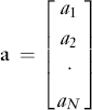
For example, we know that a portfolio's excess return will be affected by what can be different characteristics or attributes that affect all asset prices. A few examples would be the price-earnings ratio, market capitalization, and industry. Let's denote for a particular attribute a column vector, a, that shows the exposure of each risky asset to that attribute, denoted a_n:

O.1.2 Matrices

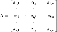
A n×m matrix is a bi-dimensional ordered array of n×m numbers. Matrices are usually indicated with boldface uppercase letters. Thus, the generic matrix A is a n×m array of the form:

Note that the first subscript indicates rows while the second subscript indicates columns. The entries a_ij—called the elements of the matrix A—are the numbers at the crossing of the i-th row and the j-th column. The commas between the subscripts of the matrix entries are omitted when there is no risk of confusion: a_{i, j} ≡ a_ij. A matrix A is often indicated by its generic element between brackets:

where the subscripts nm are the dimensions of the matrix.

There are several types of matrices. First, there is a broad classification of square and rectangular matrices. A rectangular matrix can have different numbers of rows and columns; a square matrix is a rectangular matrix with the same number n of rows as of columns. Because of the important role that they play in applications, we focus on square matrices in the next section.

O.2 SQUARE MATRICES

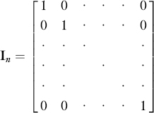
The n×n identity matrix, indicated as the matrix I_n, is a square matrix whose diagonal elements (i.e., the entries with the same row and column suffix) are equal to one while all other entries are zero:

A matrix whose entries are all zero is called a zero matrix.

A diagonal matrix is a square matrix whose elements are all zero except the elements on the diagonal:

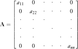
Given a square n×n matrix A, the matrix dg A is the diagonal matrix extracted from A. The diagonal matrix dg A is a matrix whose elements are all zero except the elements on the diagonal, which coincide with those of the matrix A:

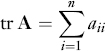
The trace of a square matrix A is the sum of its diagonal elements:

A square matrix is called symmetric if the elements above the diagonal are equal to the corresponding elements below the diagonal: a_ij = a_ji. A matrix is said to be a skew-symmetric if the diagonal elements are zero and the elements above the diagonal are the opposite of the corresponding elements below the diagonal: a_ij = a_ji, i ≠ j, a_ii = 0.

The most commonly used symmetric matrix in financial economics and econometrics is the covariance matrix, also referred to as the variance-covariance matrix. For example, suppose that there are N risky assets and that the variance of the excess return for each risky asset and the covariances between each pair of risky assets are estimated. As the number of risky assets is N, there are N² elements, consisting of N variances (along the diagonal) and N² − N covariances. Symmetry restrictions reduce the number of independent elements. In fact, the covariance between risky asset i and risky asset j will be equal to the covariance between risky asset j and risky asset i. Hence, the variance-covariance matrix is a symmetric matrix.

O.3 DETERMINANTS

Consider a square, n×n, matrix A. The determinant of A, denoted |A|, is defined as follows:

where the sum is extended over all permutations (j₁,…, j_n) of the set (1,2,…, n) and t(j₁,…, j_n) is the number of transpositions (or inversions of positions) required to go from (1,2,…, n) to (j₁,…,j_n). Otherwise stated, a determinant is the sum of all products formed taking exactly one element from each row with each product multiplied by (−1)^tj1,…,j_n). Consider, for instance, the case n = 2, where there is only one possible transposition: 1,2→2,1. The determinant of a 2×2 matrix is therefore computed as follows:

Consider a square matrix A of order n. Consider the matrix M_ij obtained by removing the ith row and the jth column. The matrix M_ij is a square matrix of order (n-1). The determinant |M_ij| of the matrix M_ij is called the minor of a_ij. The signed minor (−1)(ⁱ+j) |M_ij| is called the cofactor of a_ij and is generally denoted as α_ij.

A square matrix A is said to be singular if its determinant is equal to zero. A n×m matrix A is of rank r if at least one of its (square) r- minors is different from zero while all (r + 1)- minors, if any, are zero. A non-singular square matrix is said to be of full rank if its rank r is equal to its order n.

O.4 SYSTEMS OF LINEAR EQUATIONS

A system of n linear equations in m unknown variables is a set of n simultaneous equations of the following form:

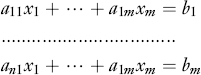
The n×m matrix:

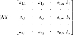
formed with the coefficients of the variables is called the coefficient matrix. The terms b_i are called the constant terms. The augmented matrix [Ab]—formed by adding to the coefficient matrix a column formed with the constant term—is represented below:

If the constant terms on the right side of the equations are all zero, the system is called homogeneous. If at least one of the constant terms is different from zero, the system is said to be non-homogeneous. A system is said to be consistent if it admits a solution, that is, if there is a set of values of the variables that simultaneously satisfy all the equations. A system is referred to as inconsistent if there is no set of numbers that satisfy the system equations.

Let's first consider the case of non-homogeneous linear systems. The fundamental theorems of linear systems state that:

An immediate consequence of the two fundamental theorems is that (1) a system of n equations in n unknown variables admits a solution and (2) the solution is unique if and only if both the coefficient matrix and the augmented matrix are of rank n.

Let's now examine homogeneous systems. The coefficient matrix and the augmented matrix of a homogeneous system always have the same rank and thus a homogeneous system is always consistent. In fact, the trivial solution x₁ = … = x_m = 0 always satisfies a homogeneous system.

Consider now a homogeneous system of n equations in n unknowns. If the rank of the coefficient matrix is n, the system has only the trivial solution. If the rank of the coefficient matrix is r < n, then Theorem 2 ensures that the system has a solution other than the trivial solution.

O.5 LINEAR INDEPENDENCE AND RANK

Consider an n×m matrix A. A set of p columns extracted from the matrix A:

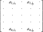
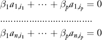
are said to be linearly independent if it is not possible to find p constants β_s, s = 1,…, p such that the following n equations are simultaneously satisfied:

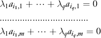
Analogously, a set of q rows extracted from the matrix A are said to be linearly independent if it is not possible to find q constants λ_s, s = 1,…, q such that the following m equations are simultaneously satisfied:

It can be demonstrated that in any matrix the number p of linearly independent columns is the same as the number q of linearly independent rows. This number is equal, in turn, to the rank r of the matrix. Recall that a n×m matrix A is said to be of rank r if at least one of its (square) r- minors is different from zero while all (r + 1)-minors, if any, are zero. The constant p, is the same for rows and for columns. We can now give an alternative definition of the rank of a matrix:

Given a n×m matrix A, its rank, denoted rank (A), is the number r of linearly independent rows or columns as the row rank is always equal to the column rank.

O.6 VECTOR AND MATRIX OPERATIONS

Let's now introduce the most common operations performed on vectors and matrices. An operation i s a mapping that operates on scalars, vectors, and matrices to produce new scalars, vectors, or matrices. The notion of operations performed on a set of objects to produce another object of the same set is the key concept of algebra. Let's start with vector operations.

O.6.1 Vector Operations

The following three operations are usually defined on vectors: transpose, addition, and multiplication.

O.6.1.1 Transpose

The transpose operation transforms a row vector into a column vector and vice versa. Given the row vector x = [x₁,…, x_n] its transpose, denoted as x^T or x′, is the column vector:

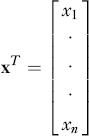
Clearly the transpose of the transpose is the original vector: (x^T)^T = x.

O.6.1.2 Addition

Two row (or column) vectors x = [x₁,…, x_n], y = [y₁,…, y_n] with the same number n of components can be added. The addition of two vectors is a new vector whose components are the sums of the components:

x + y = [x₁ + y₁,…, x_n + y_n]

This definition can be generalized to any number N of summands:

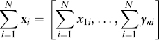
The summands must be both column or row vectors; it is not possible to add row vectors to column vectors.

It is clear from the definition of addition that addition is a commutative operation in the sense that the order of the summands does not matter: x + y = y + x. Addition is also an associative operation in the sense that x + (y + z) = (x + y) + z.

O.6.1.3 Multiplication

We define two types of multiplication: (1) multiplication of a scalar and a vector and (2) scalar multiplication of two vectors (inner product).²

The multiplication of a scalar a and a row (or column) vector x, denoted as ax, is defined as the multiplication of each component of the vector by the scalar:

ax = [ax₁,…, ax_n]

A similar definition holds for column vectors. It is clear from this definition that:

||ax|| = |a| ||k||

and that multiplication by a scalar is associative as:

||a(x + y)|| = ||ax|| + ||ay||

The scalar product (also called the inner product), of two vectors x, y, denoted as x · y, is defined between a row vector and a column vector. The scalar product between two vectors produces a scalar according to the following rule:

Two vectors x, y are said to be orthogonal if their scalar product is zero.

O.6.2 Matrix Operations

Let's now define operations on matrices. The following five operations on matrices are usually defined: transpose, addition, multiplication, inverse, and adjoint.

O.6.2.4 Transpose

The definition of the transpose of a matrix is an extension of the transpose of a vector. The transpose operation consists in exchanging rows with columns. Consider the n×m matrix A = {a_ij}_nm. The transpose of A, denoted A^T or A′ is the m×n matrix whose ith row is the ith column of A:

A^T = {a_ji}_mn

The following should be clear from this definition:

(A^T)^T = A

and that a matrix is symmetric if and only if:

A^T = A

O.6.2.5 Addition

Consider two n×m matrices A = {a_ij}_nm and B = {b_ij}_nm. The sum of the matrices A and B is defined as the n×m matrix obtained by adding the respective elements:

A + B = {a_ij + b_ij}_nm

Note that it is essential for the definition of addition that the two matrices have the same order n×m.

The operation of addition can be extended to any number N of summands as follows:

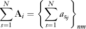
where a_sij is the generic i, j element of the sth summand.

O.6.2.6 Multiplication

Consider a scalar c and a matrix A = {a_ij}_nm. The product cA = Ac is the n×m matrix obtained by multiplying each element of the matrix by c:

cA = Ac = {ca_ij}_nm

Multiplication of a matrix by a scalar is associative with respect to matrix addition:

c(A + B) = cA + cB

Let's now define the product of two matrices. Consider two matrices A = {a_it}_np and B = {b_sj}_pm. The product C = AB is defined as follows:

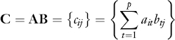
The product C = AB is therefore a matrix whose generic element {c_ij} is the scalar product of the ith row of the matrix A and the jth column of the matrix B. This definition generalizes the definition of scalar product of vectors: The scalar product of two n-dimensional vectors is the product of a 1−n matrix (a row vector) for a n−1 matrix (the column vector).

O.6.2.7 Inverse and Adjoint

Consider two square matrices of order nA and B. If AB = BA = I, then the matrix B is called the inverse of A and is denoted as A⁻¹. It can be demonstrated that the two following properties hold:

Consider now a square matrix of order nA = {a_ij} and consider its cofactors α _ij. Recall that the cofactors α_ij are the signed minors (−1)(^ij) |M_ij| of the matrix A. The adjoint of the matrix A, denoted as Adj(A), is the following matrix:

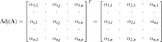
The adjoint of a matrix A is therefore the transpose of the matrix obtained by replacing the elements of A with their cofactors.

If the matrix A is non-singular, and therefore admits an inverse, it can be demonstrated that:

A square matrix of order nA is said to be orthogonal if the following property holds:

AA′ = A′A = I_n

Because in this case A must be of full rank, the transpose of an orthogonal matrix coincides with its inverse: A⁻¹ = A′

O.7 EIGENVALUES AND EIGENVECTORS

Consider a square matrix A of order n and the set of all n-dimensional vectors. The matrix A is a linear operator on the space of vectors. This means that A operates on each vector producing another vector subject to the following restriction:

A(ax + by) = aAx + bAy

Consider now the set of vectors x such that the following property holds:

Ax = λx

Any vector such that the above property holds is called an eigenvector of the matrix A and the corresponding value of λ is called an eigenvalue.

To determine the eigenvectors of a matrix and the relative eigenvalues, consider that the equation Ax = λx can be written as:

(A − λI)x = 0

which can, in turn, be written as a system of linear equations:

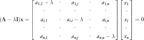
This system of equations has non-trivial solutions only if the matrix A λI is singular. To determine the eigenvectors and the eigenvalues of the matrix A we must therefore solve the equation:

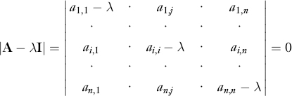
The expansion of this determinant yields a polynomial ø(λ) of degree n known as the characteristic polynomial of the matrix A. The equation ø(λ) = 0 is known as the characteristic equation of the matrix A. In general, this equation will have n roots λ_s, which are the eigenvalues of the matrix A. To each of these eigenvalues corresponds a solution of the system of linear equations as illustrated below:

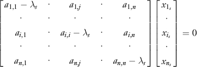
Each solution represents the eigenvector x_s corresponding to the eigenvector λ _s. As explained in Chapter 15 as well as in Web-Appendix P, the determination of eigenvalues and eigenvectors is the basis for principal component analysis.