WEB–APPENDIX P

PRINCIPAL COMPONENT ANALYSIS IN FINANCE

In Chapter 15, we discussed principal component analysis (PCA). This statistical tool is widely used in finance. It is useful not only for estimating factor models here, but also for extracting a few driving variables out of many for the covariance matrix of asset returns. Hence, it is important to understand the statistical intuition behind it. To this end, we provide a simple introduction in this appendix.

Perhaps the best way to understand PCA is to go through an example in detail. Suppose there are two risky assets, whose returns are denoted by and , with covariance matrix:

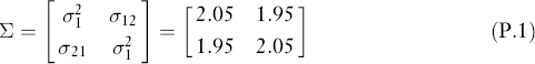
That is, we assume that they have the same variances of 2.05 and covariance of 1.95. Our objective is to find a linear combination of the two assets so that it has a large component in the covariance matrix, as will be clear below. For notational brevity, we assume first that the expected returns are zeros, that is,

and will relax this assumption at the end of this section.

Recall that we call any vector (a₁, a₂)′ satisfying:

an eigenvector of σ, and the associated λ the eigenvalue. In our example here, it is easy to verify that:

and

so 4 and 0.1 are the eigenvalues, and (1,1)′ and (1, −1)′ are the eigenvectors.

In practice, computer software is available to compute the eigenvalue and eigenvectors of any covariance matrix. The mathematical result is that for a covariance matrix of N assets, there are exactly N different eigenvectors and N associated positive eigenvalues (these eigenvalues can be equal in some cases). Moreover, the eigenvectors are orthogonal to each other; that is, their inner product or vector product is zero. In our example, it is clear that:

It should be noted that the eigenvalue associated with each eigenvector is unique, but any scale of the eigenvector remains an eigenvector. In our example, it is obvious that a double of the first eigenvector, (2,2)′, is also an eigenvector. However, the eigenvectors will be unique if we standardize them, making the sum of the elements be 1. In our example,

are the standardized eigenvectors, which are obtained by scaling the earlier eigenvectors by . These are indeed standardized, since:

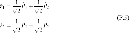
Now let us consider two linear combinations (or portfolios without imposing the weights summing to 1) of the two assets whose returns are and ,

where . Both and are called the principal components (PCs). There are three important and interesting mathematical facts about the PCs.

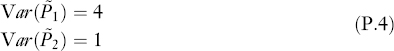
1. • Fact 1. The variances of the PCs are exactly equal to the eigenvalues corresponding to the eigenvectors used to form the PCs.

   That is,

   

   Note that the two PCs are random variables since they are the linear combination of random returns. So, their variances are well defined. The equalities to the eigenvalues can be verified directly.

2. • Fact 2. The returns can also be written as a linear combinations of the PCs.

   The PCs are defined as linear combinations of the returns. Inverting them, the returns are linear functions of the PCs too. Mathematically, and so Since A is orthogonal, A⁻¹ = A′, thus . That is, we have:

   

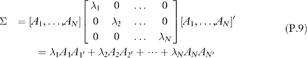
3. • Fact 3. The asset return covariance matrix can be decomposed as the sum of the products of eigenvalues with the cross products of eigenvectors.

Mathematically, it is known that:

which is also easy to verify in our example. The economic interpretation is that the total risk profile of the two assets, as captured by their covariance matrix, is a sum of two components. The first component is determined by the first PC, and the second is determined by the second PC. In other words, in the return linear combinations, equation (P.5), if we ignore P₂, we will get only λ₁A₁A₁′, the first component in the covariance matrix decomposition, and only the second if we ignore P₁. We of course obtain the entire Σ if we ignore neither.

The purpose of the PCA is finally clear. Since 4 is 40 times as big as 0.1, the second component in the σ decomposition has little impact, and hence may be ignored. Then, ignoring , we can write the returns simply as, based on equation (P.5),

This says that we can reduce the analysis of and by analyzing simple functions of . In this example, the result tells us that the two assets are almost the same. In practice, there may be hundreds of assets. By using PCA, we can reduce the dimensionality of the problem substantially to an analysis of perhaps a few, say five, PCs.

In general, when there are N assets with return computer software can be used to obtain the N eigenvalues and N standardized eigenvectors. Let λ₁≥λ₂≥…≥λ_N ≥ 0 be the N eigenvalues in decreasing order, and A_i = (a_i1, a_i2,…, a_iN)′ be the standardized eigenvector associated with λ_i, and A be an N × N matrix formed by the all the eigenvectors. Then, the i-th PC is defined as , all of which can be computed in matrix form,

The decomposition for σ is:

It is usually the case that, for some K, the first K eigenvalues are large, while the rest are small, and can then be ignored. In such situations, based on the first K PCs, we can approximate the asset returns by:

In most studies, the K PCs may be interpreted as K factors that (approximately) derive the movements of all the N returns. Our earlier example is a case with K = 1 and N = 2.

In the above PCA discussion, the expected returns of the asset are assumed to be zero. If they are nonzero and given by a vector (μ₁,μ₂,…,μ _N)′, σ will remain the same, and so will the eigenvalues and eigenvectors. However, in this case we need to replace all the in equation (P.8) by , and add μ_i's on the right-hand side of equation (P.10). The interpretation will be, of course, the same as before.

In Case 1 of the factor model estimation (i.e., known or observable factors) in Section 15.4.1 in Chapter 15, the K PCs clearly provide a good approximation of the first K factors since they explain the asset variations the most given K. Moreover, in either Case 1 or Case 2 (latent factors), the PCA is equivalent to minimizing the model errors, as given by equation (15.34) in Chapter 15, by choosing both the loadings and factors, and hence, the solution should be close to the true factors and loadings.