11

RISK AND RISK MANAGEMENT

What do financial economists mean by risk and how is risk to be managed? In this chapter, we explain why risk cannot be described in the abstract, but instead depends on such specifics as the decision maker's preferences, wealth position, and, in many cases, on environmental circumstances as well. For example, a possible monetary loss of $1,000 can mean a great deal to a struggling student, but much less to a wealthy businessperson. Similarly, a possible loss of $1,000 is more serious in a depressed economy than in a buoyant one. Risks can also be characterized according to a number of other features. For example, risks can differ with the decision maker's chosen time horizon. Moreover, those risks can evolve dynamically through time. Decision makers’ preferences can also change, both with respect to differing circumstances and over time. As a result of these many factors characterizing risk, management tasks also take on a large variety of forms that may similarly change through time.

In order to present the complexities of risk-management tasks systematically, this chapter approaches them as management problems. We begin the chapter by outlining different kinds of risks and the attitudes of decision makers facing them. We then examine how different combinations of these elements present a variety of optimization problems. In the present discussion, optimization means doing the best you can, given what you already know and what you can find out.¹ While this concept of optimization includes the concept of expected utility maximization, it goes further. Under uncertainty, for example, maximizing choices are ruled out by definition: Uncertainty is taken to refer to situations where it is not possible to attach probability distributions to possible outcomes. But even under uncertain circumstances, attempting to make good rather than poor decisions is still a sensible goal.

The chapter proceeds by defining differences between risk and uncertainty. Then the decision makers’ management objectives and the criteria they employ in pursuing those objectives are considered. Once a criterion has been chosen, and assuming the decision maker has some ability to affect the situation being faced, the chapter discusses how the criterion can be used to guide the choice of decisions. For example, a decision maker may be able to formulate a problem under risk as one of maximizing the expected utility of a pre-selected utility function by choosing among risk transfer methods.

In this chapter, different aspects of probability distributions are considered. Moreover, specifically, we (1) describe some of the main features of the probability distributions that decision makers are likely to encounter in practice, (2) discuss how different probability distributions can be incorporated in problem formulations, and (3) examine how the distributions can affect problem solutions. Finally, different forms of utility functions and how choices of utility functions can affect solutions to risk-management problems are explained.

11.1 RISK AND UNCERTAINTIES

While the difference between uncertainty and risk can be stated as a matter of degree, for discussion purposes it is convenient to distinguish the two situations more sharply. Furthermore, uncertainty itself can be divided into two classifications, the first of which refers to situations where qualitative descriptions are so difficult to generate that it is not practical even to define possible future states of the world. The second kind of uncertainty (and the one usually addressed in the financial economics literature) refers to situations in which it is possible to define future states of the world, but not to attach probability distributions to their possible realizations.² Risk refers to situations in which it is possible both to define future states of the world and the probabilities³ with which they might occur. As we have already stated, the categories are matters of degree: It is not easy, or in some circumstances even possible, to distinguish sharply between the two forms of uncertainty, nor is it easy to distinguish between uncertainty and risk. From a problem-solving point of view, distinguishing between types of uncertainty depends on how practically useful it is to define possible future states of the world, and distinguishing risk from uncertainty depends on how practically useful it is to estimate and employ a probability distribution of state outcomes.

Whatever the form of uncertainty or risk faced, the decision maker starts out by considering how the management problem can be modeled, including how decisions can affect the impact of outcomes. That is, decision makers attempt to foresee possible outcomes, structure them, and, if possible, assess their impacts. Depending on the extent of a decision maker's capabilities and knowledge of a situation, the decision maker may adopt different management techniques.

11.1.1 Uncertainty

The first kind of uncertainty is the most difficult to describe and also the most difficult to deal with. It can arise, for example, in such circumstances as new product development. If the success of a product is likely to be affected by the unknown reactions of both consumers and competitive producers, it may well be difficult to define relevant future states of the world with any useful degree of precision. At the same time, attitudes towards the uncertainties cannot be very precisely specified either, not least because the circumstances themselves are not very well defined. As a result, some decision makers might simply decide to avoid such situations.

However, if a decision maker decides to proceed and attempts to manage a situation like that of new product development, the choice of suitable criteria may be relatively crude. For example, the decision maker may attempt either to avoid some of the uncertainties or attempt to control possible losses.⁴ To help formulate alternative possible actions, the decision maker might attempt to determine key aspects of the new product's acceptance by consumers, as well as to determine key aspects of competitor reactions. One consideration in deciding to face uncertainty of the first kind might be that losing out to competitors is regarded as an unacceptable outcome. If so, the best the decision maker might be able to do is to go ahead with a (necessarily sketchy) development plan, and simultaneously formulate an exit strategy if things work out badly.

The second type of uncertainty, and the type that is most frequently described in the literature, can be represented by a decision tree that outlines the possible outcomes of a situation (see Chapter 10 for an example). However, by definition uncertainty means it is not practically useful to attempt to attach probabilities to the outcomes.⁵ For example, a large financial institution might face bankruptcy if certain asset markets fail to function smoothly. In analyzing these prospects, management of the financial institution might be able to establish possible loss magnitudes in several lines of business, yet still be unable to describe the outcomes probabilistically.⁶ In such situations decision makers are likely to place considerable emphasis on loss prevention, possibly attempting to avoid what are seen to be the worst outcomes. For example, in the uncertain world financial environment starting in the summer of 2007, one common response to uncertainty was simply to avoid certain kinds of transactions. This strategy, mainly expressed through purchases of assets viewed as having little credit risk, is often referred to as a “flight to quality.”

It is important to bear in mind that uncertain situations can evolve through time, as can decision makers’ capabilities for addressing them.⁷ Consequently, in practice, managing uncertainty is a dynamic process. It is also important to bear in mind that decision makers can err in their modeling efforts, so that the situations they attempt to address differ from the situations they actually face. This is known as modeling risk.

11.1.2 Risk

The bulk of the financial economics literature focuses on quantitative approaches that permit structuring and analyzing choices intended to affect the impacts of future state realizations. Situations under risk are usually modeled as maximization problems, and can very often be analyzed to good effect using decision trees. (Again see Chapter 10 for an example.) The decision maker's attitudes toward risk may be represented by one of the utility functions introduced in Chapter 9.⁸ Another way of incorporating attitudes toward risks is to value outcomes using risk-neutral probability measures, as will be discussed in Chapter 16. Finally, still other criteria such as chance-constrained approaches may be used, as discussed further below.

11.2 DECISION CRITERIA

The possible choices of criteria stem from an interaction between the decision maker and the kind of situation being faced. We have already mentioned how relatively informal criteria may be chosen under conditions of uncertainty. Under risk, decision makers’ criteria include expected wealth maximization, minimizing maximum regret, and the customary expected utility maximization. Different choices of criteria will help manage certain aspects of a risk-management problem, but the solutions will not necessarily be consistent with those obtained using other criteria. In fruitfully managing either risks or uncertainties, it may be as important to recognize the implications of criterion choice as it is to formulate other aspects of the problem as clearly and as comprehensively as possible.

11.2.1 Wealth-Based and Dispersion-Based Criteria

Wealth-based criteria emphasize the distribution of a decision maker's final wealth, usually focusing on such measures of central tendency as expected value. For example, an expected utility-maximizing, risk-neutral decision maker would choose between two portfolios on the basis of their expected outcomes (or expected returns), without regard to any other features of the outcome distribution.

Dispersion-based criteria emphasize the spread of a random variable. For example, the variance of final wealth and the variance of the ratio of the return to invested wealth are both measures of dispersion about the mean. They are also both symmetric measures, and as a result consider variation above the mean as serious as variation below the mean. In contrast, many decision makers prefer to use criteria that weight losses more heavily than gains.⁹

Both wealth-based and dispersion-based criteria can give conflicting results. For example, a nonsatiable decision maker would prefer to end up with a wealth distribution that offers outcomes of either of say $2 or $4 with equal probability rather than with a certain outcome of $1. However, a measure of dispersion considered by itself would point to choosing the certain wealth of $1, since that outcome has zero dispersion while the first lottery's dispersion is positive. To resolve these difficulties, measures of final wealth and measures of dispersion may both be incorporated in choosing a criterion function. For example, it is not uncommon to find decision makers using a utility function such as:

E(X) − βσ²(X)

where β > 0 is used to reflect a degree of risk aversion,¹⁰ while the risk of X is measured by the variance σ²(X).¹¹

11.2.2 Target-Based Criteria

In some instances, management may exhibit risk aversion through attempts to avoid downside risk (unfavorable outcomes). We shall refer to techniques of this type as target-based approaches or chance-constrained approaches. The notions are perhaps most easily expressed in terms of an example.

Suppose the management of a firm is trying to allocate liquid assets to two accounts, one of which (e.g., a bank checking account) is riskless but pays no interest, while the other offers a risky return (money market investments, for example, if we assume they will not necessarily be held to maturity). For simplicity we assume the rate of return r on the second account is uniformly distributed over the range [20.5, 0.7]. If R is the amount currently available for allocation to the two accounts, the value of invested resources next period will be:

where S is invested in the risky asset and the remainder R − S is kept in the non-interest-bearing riskless account. Note that for simplicity that equation (11.1) can be rewritten as:

Now suppose management would like to make the next period investment value as large as possible but subject to the condition that R) Sr not fall below 95% (an arbitrarily chosen percentage) of the original value of R too often. Of course, this means we also have to define “ too often.” In this example we mean that if the investment falls below 95% of its original value, it should not do so more than 25% of the time (another arbitrary choice). In other words, management does not wish to find the firm in an illiquid position (having lost more than 5% of the original investment value) more than 25% of the time. Formally, this can be expressed by saying that management wishes to:

subject to:

Pr[R + Sr ≥ 0.95R] ≥ 0.75 and 0 ≥ S ≥ R

where Pr means cumulative probability.

Equation (11.3) says that we should maximize expected return subject to a (probabilistic) minimum balance requirement calculated at the end of the period. This problem may be rewritten in a somewhat simpler form as:

subject to:

where α = S/R. (The solution to this problem is α* = 0.25.)

The constraint requiring that downside risk be controlled according to equation (11.3) imposes an opportunity cost on the firm, since if more risk were taken, expected return would be higher. One way of assessing this opportunity cost is to allow the probability of losses to increase and recalculate the solution to the original problem. (Another way is to allow for larger losses but with the same probability.) To allow for a larger loss probability, we replace the constraint in (11.4) by

Pr[(1 + α r) ≥ 0.95 ≥ 0.67 and 0 ≥ α ≥ 1

The solution to this problem is α* = 0.50. The solution allows the expected return on invested assets to rise to 0.05, but the standard deviation of return also rises. Without further information, it is not possible to say which distribution management ought to choose, but at least the calculations make explicit the trade-offs between risk (in this case, risk of decreased liquidity) and return. Moreover, we have shown that when practical problems arise (for which only a rough risk-return trade-off calculation is required), the chance-constrained approach may provide a useful way of examining the trade-offs involved.

11.2.3 Criterion Choice

As mentioned in Chapter 9, expected utility has been offered as a financial decision criterion since the time of Daniel Bernoulli. Moreover, analyses that use other criteria may turn out to be consistent with maximizing expected utility. First, the use of risk-neutral probabilities to calculate the value of a decision can be wholly consistent with expected utility maximization, as will be shown in Chapter 16. As a second example, minimizing the probability of missing a target such as the one described above can also be shown to be consistent with maximizing the expectation of a particular form of utility function.¹²

Some financial research replaces the classic von Neumann Morgenstern wealth-dependent utility function with more elaborate forms that offer greater flexibility in representing the consequences of choices. For example, state-dependent utility functions are utility functions like those introduced in Chapter 9, but are more complex in that they score outcomes according to both wealth and the state in which wealth is received. That is, the utility function is written as u (w, s) where w represents wealth and s represents individual states drawn from a set of possible states S. Research using state-dependent utilities is capable of explaining a number of observed asset price features that will be discussed in later chapters in this book.¹³

11.3 METHODS OF RISK TRANSFER

Risk management often involves transferring risks to the agents best equipped to bear them. Risk transfer can make it possible for agents to undertake new risks that they would otherwise avoid, and hence improve an economy's resource allocation. Many attempts to manage risks involve selecting among forms of risk transfer according to a pre-selected criterion. Using the notion of a decision tree to represent the management problem, one can think of risk transfers as actions intended to affect the impacts of certain outcomes.¹⁴ The forms of risk transfer considered next are hedging, insurance, and diversification.¹⁵ In many, but not necessarily all, such analyses we assume the outcomes themselves are not capable of being changed, and we assume further that the probabilities of realizing the outcomes do not react to our choice of risk transfer method. Although most of the agents discussed below are modeled as transferring risks to other parties, their ability to do so depends on the existence of agents who willingly act as counterparties to assume the risks.

11.3.1 Hedging

Hedging means eliminating the possibility of realizing either a gain or a loss. A hedge can be arranged either by selling the risky prospect to another party, or by buying an offsetting risky prospect. For example, suppose a decision maker has a long position in a random variable X that promises to pay $4 with probability¹/2 and 2$2 with probability¹/2. If the decision maker now sells short the same random variable, that position becomes X − X, offering a certainty outcome of zero irrespective of the outcome of X. In such a situation the decision maker is said to be fully hedged against the risk. The decision maker has, of course, eliminated the potential for either loss or gain in this example. If the offsetting short position is to be arranged through a market transaction, the hedger must be able to find a suitable counterparty—say, a speculator who might assume a long position in X.

Hedging is a form of risk management that involves risk sharing. We will discuss financial instruments, called derivatives, that can be used for hedging and other forms of risk management in Chapters 18 and 19.

11.3.2 Insuring

Insuring means reducing the probability of one or more downside outcomes by buying insurance protection. The price paid for the protection is referred to as an insurance premium. Upside outcomes are not usually affected by the purchase of insurance.

To see the difference between hedging and insuring, consider a variant on the above example. Suppose it is now possible to purchase, for price p, an insurance contract P that allows the insured to sell to the insurance company the variable X at a price of $1.5. The decision maker's payoffs, exclusive of the insurance premium p, are then:

The decision maker's loss exposure has now been reduced from $2 to $0.5, by paying a price of p, so that if things turn out badly, the decision maker's total loss is $0.5 + p. On the other hand, the decision maker's gross gain remains at $4, and the net gain including the insurance premium (represented by the cost of the insurance contract, in this case a put) is $4 − p. As in the hedging example above, the risk transfer can only be brought about if a counterparty can be found to assume the risk. In this case, the counterparty is the agent who sells the insurance contract P at the assumed price p.

In Chapters 18 and 19 we further distinguish insurance-type contracts from risk-sharing type contracts used for risk management. We describe an insurance-type contract in Chapter 19.

11.3.3 Diversifying

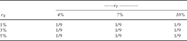
Diversifying means combining different prospects in ways designed to reduce downside risks. To see how diversification can lower risk in relation to return, consider investing in just two finanical instruments, X and Y. Denoting realized returns on the two financial instruments by r_X and r_Y, Table 11.1 shows the joint probabilities, estimated at time 0, with which the returns might be realized one period later. For example, the joint outcome r_X = 1%, r_Y = 10% is assumed to occur with probability 1/9, as are all the other combinations shown in the table.

TABLE 11.1 JOINT PROBABILITIES OF RETURNS

The expected return on either financial instrument in Table 11.1 is given by the sum of the outcomes multiplied by the probability of realizing each possible outcome. The probabilities of the outcomes of r_X are given by the row sums of the joint probabilities, while the probabilities of the outcomes of r_Y are given by the column sums of the joint probabilities. Thus,

E(r_X) = (1/3)(0.01) + (1/3)(0.03) +(1/3)(0.05) = 0.03

and E (r_Y) = 0.07.

The variance of returns, and its square root the standard deviation, are both measures of how dispersed returns can be—the greater the dispersion, the greater the variance, and hence also the standard deviation. The variance is defined as the expected value of the square of the differences between outcomes and their mean:

Var(r_X) = σ²(r_X) = E[r_X − E(r_X)]²

For example, letting σ²(r_X) denote the variance of return on financial instrument X,

For subsequent use, note that the standard deviation of return on financial instrument X is σ(r_X) = (0.000267)^½. Similar calculations show that σ(r_Y) = (0.0006)^½.

Since the two financial instruments X and Y offer expected returns of 0.03 and 0.07, respectively, any portfolio combining them will have an expected return equal to the weighted average of the two. For example, a portfolio constructed by investing half the available funds in each of the two financial instruments has an expected return equal to:

(1/2)[E(r_X) + E(r_Y) = 0.05

The variance of return for a portfolio composed of the two risky financial instruments is given by the formula:

where

In the present example this covariance is equal to zero because the two returns for the financial instruments are distributed independently. You can see the returns are statistically independent by noting that regardless of which outcome you consider for r_X, the probabilities of the three outcomes for r_y are all equal.¹⁶

11.4 CHARACTERISTICS OF PROBABILITY DISTRIBUTIONS

An important assumption in finance theory is the probability distribution assumed for asset returns. Unfortunately, the probability distribution traditionally used in financial theory and the one that dominates statistics textbooks used in business schools—the normal distribution—does not correspond closely with the distributions typically found in real-world financial markets.¹⁷ Although in principle any form of probability distribution can be incorporated in a decision-tree analysis, in practice the best choice of probability distribution is not always easy to determine.¹⁸ First, there are many candidate distributions that have to be considered in formulating a risk-management problem. In particular, statistically convenient choices of distributions may simplify modeling the problem, but may also give inaccurate descriptions of the probabilities with which states might be realized. Moreover, estimating the appropriate distribution may be subject to error, and any such errors affect model solutions. Finally, estimating and using a realistic form of probability distribution can involve a considerable amount of computation, an important practical consideration in managing institutional portfolios where large numbers of financial instruments must be valued frequently.¹⁹

As just explained, financial economics usually assumes that asset returns are normally distributed. Since the normal distribution can be described by two parameters—its mean and its variance—portfolio risk-return relationships (see Chapters 13 and 14) can also be described using the same two parameters.²⁰ While assuming that portfolio risks and returns can thus be modeled, the appropriateness of using the assumption has been investigated empirically and found wanting. Estimated returns turn out not be normally distributed. Rather, the estimated distributions

1. possess heavier tails (i.e., fat tails) than those of the normal distribution
2. are skewed rather than symmetric (i.e., E{[X − E(X)]³} ≠ 0) and
3. may possibly be leptokurtic (i.e., the fourth moment about the mean E{[X E − (X)]⁴} > 3, its value for the normal distribution).

In addition, empirical distributions can have extreme realizable outcomes with higher probability than is reflected even by popular choices of heavy-tailed distributions.

The skewness parameter has a particularly important impact on portfolios that include such instruments as options (see Chapters 18 and 19), but even recognizing the effects of skewness may not be sufficient to capture all important problem features. A correct analysis can involve working with multivariate distributions whose features are described by the statistical (marginal) properties of all the component random variables in the portfolio. Moreover, the dependence structures among components are likely to be more complex than those capable of being captured by the linear correlation coefficients used in Section 11.3. The distributions needed for full analysis may have to incorporate such features as how different risks combine, how their component dependencies can change through time, and consequently how the entire portfolio's distribution can change through time.

Models can be constructed to display all these realistic features, but they can be both costly to construct and difficult to solve. For example, if one tried to capture all of the foregoing features using decision-tree analyses, the resulting problem representation might be very complex. Indeed, some models are so complex that even today's fastest computers cannot determine solutions to them in short periods of time. For example, the daily marking to market of an institutional portfolio containing thousands of securities can, if carried out fully, actually require more time than is available between trading periods.

11.5 EXPECTED UTILITY THEORY AND ARROW-PRATT RISK AVERSION

Just as the choice of probability distribution affects the solution to a risk-management problem, so does the choice of criterion function. This section examines how some properties of utility functions affect the solutions they imply. In Chapter 9 we explained that the utility function of a risk averter is concave, and introduced the measure known as the Arrow-Pratt risk aversion coefficient. We continue that investigation here.

An intuitive way to characterize a risk averter's behavior is to say that downside risk is regarded more seriously by a risk averter than an equal upside potential is valued, meaning that the risk-averse investor requires to be compensated if she is to accept risk. To see how upside potential and downside risk are weighted by a risk-averse investor, consider the lottery X: payoff of $10 and 2$10 with equal probability. This lottery's mean is zero. One can calculate the certainty equivalent value for this lottery, which is defined as an amount of cash, paid or received with certainty, that the decision maker regards as just equal to the value of the lottery. Hence, a risk-averse investor's certainty equivalent value for lottery X will be negative. In the present example (continuing with the practice of not including dollar signs in the utility function),

where c is the certainty equivalent value of the lottery and ““means “is defined to be.” As already explained, in the case of this example c is a negative number for any risk averter. If the individual were only made as unhappy by downside risk (moving from 0 to − 10) as he would be made happier by upside potential (moving from 0 to 10), the certainty equivalent value of the lottery would be zero. But since it is in fact negative, downside risk must be weighted more heavily by an investor who is a risk averter. This situation suggests that the risk-averse investor might be willing to give up some amount of wealth in order to avoid this particular lottery. The maximum amount of wealth that would thus be given up is called a risk premium.²¹ As a general matter, the amount of the risk premium depends on both the lottery and the precise nature of the utility function.

Recall from Chapter 9 that both risk premia and some aspects of risk-taking behavior can be related to characteristics of utility functions known as the Arrow-Pratt measures of local risk aversion. To see this, let us again consider our hypothetical risk-averse investor, now with an initial wealth endowment of w and a more generally specified lottery X. For convenience, we suppose that E[X] is still 0. We then ask what risk premium π (w, X) must be deducted from the E[X] to create a certainty equivalent level of wealth that will provide the investor with the same satisfaction as from her original position. That is, we wish to find the risk premium that satisfies

We can use a Taylor expansion around w to find a local, linear approximation of the function u(.).²² Starting with the right-hand side of equation (11.5), we shorten the notation for risk premium to π and bear in mind that E(X) = 0 by assumption. Then the Taylor expansion of u(w − π) is:

FIGURE 11.1 DOWNSIDE RISK IS MORE IMPORTANT THAN AN EQUAL UPSIDE POTENTIAL TO RISK-AVERTER

where u′ (w) is the first derivative of the utility function and O (π²) refers to a term whose magnitude is at most equal to the order of π², that is, small enough to be ignored. Similarly, the Taylor expansion of the left-hand side, E[u(W + X)], is:

and O(X³) is also assumed to be small enough to be ignored. Equation (11.7) can then be simplified as shown because E[u(w)] = u(w) (initial wealth is known with certainty) and because E(X) = 0, so that . Using equations (11.6) and (11.7), and solving for π, we obtain:

The function −u″ (w) /u′ (w) in equation (11.8) is the Arrow-Pratt measure of absolute risk aversion²³ first referred to in Chapter 9.

Since variance is always positive, the sign of the risk premium π will depend on the sign of the ratio. We have assumed that utility always increases with wealth so u′ (w) > 0. For a risk averter, utility of wealth increases at a decreasing rate as wealth increases; that is, u″ (w) < 0, and therefore u″ (w)/u′ (w) < 0. This type of utility function is shown in Figure 11.1, and for such an individual, the risk premium π > 0 as would be expected.

In a similar manner, we can show that an individual's attitude toward proportional risks is expressed by the measure of relative risk aversion:

An individual's attitude toward risks measured in monetary amounts is reflected by the measure of absolute risk aversion, as we show next. Recall that every consumer's utility may be specified as to origin and scale. If we take a particular lottery, such as a payoff of $10 with a probability of ¹/2 and a payoff of $0 with a probability of ¹/2 and define:

u_A(0) = u_B(0) = 0;u_A(10) = u_B(10) = 1

where A and B refer to two investors, and if investor B's certainty equivalent c_B for the lottery X is less than c_A, B can be said to show greater absolute risk aversion. It can be shown, moreover, that B's measure of absolute risk aversion is, in this case, larger than A's (because B's risk premium is larger).²⁴ The observation implies that when the utilities are appropriately scaled, the curvature of B's utility is greater than the curvature of A's. That is, when utilities are appropriately scaled for comparability, the measure of absolute risk aversion increases as the utilities’ curvature increases.

Another question of interest is how the absolute risk-aversion measure might change with a significant change in the level of initial wealth. It is frequently speculated on the basis of casual empiricism that absolute risk aversion should decrease as the individual's wealth increases, and that relative risk aversion might remain about constant. If absolute risk aversion decreases, it can be shown that a decision maker's investment in a lottery of fixed composition will increase. Similarly, if relative risk aversion decreases, it can be shown that a decision maker's investment in a proportional lottery of fixed composition will increase.

Such properties of utility functions and their implications for risky behavior can be inferred by calculating the Arrow-Pratt measures. For example, a quadratic utility function defined on portfolio returns has been widely used in a portfolio context, as described further in Chapter 13. Let us, following the example of Chapter 9, write a representative quadratic utility function as:

having u′(w) = a − 2bw, and u″ (w) = 2b (for w ≤ a/2b). The corresponding measures of risk aversion are:

Both of these measures are increasing functions of w rather than being decreasing or constant, thus implying that the quadratic decision maker becomes more averse to risk as wealth increases. Some observers reject the use of quadratic utility on the grounds that increasing risk aversion is a priori implausible.

The definitions of risk premium and of the risk-aversion measures provide useful ways to examine the properties of various possible utility functions and to make inferences about risky behavior, as we have just seen. Recall, though, that the definitions of absolute and relative risk aversion assume that risks are small, or local. The local property is due to the fact that the measures of risk aversion are derived using a linear Taylor expansion around the current wealth level, and such an approximation is valid for only small changes. In the next chapter, we show how a global measure of riskiness proposed by Aumann and Serrano (2008) can be related to the Arrow-Pratt measures of local risk aversion.

KEY POINTS

• The environments in which financial decisions are taken can be viewed as either uncertain or as risky.
• Uncertainty refers to an environment that is difficult to specify, even qualitatively. For example, in extreme cases it may not be possible to identify possible outcomes in even a qualitative fashion.
• In less extreme cases of uncertainty it may be possible to identify outcomes qualitatively, but not to attach a meaningful probability distribution to the outcomes (i.e., one that will be helpful in choosing among those outcomes).
• Although some quantitative approaches to modeling choices under uncertainty have been proposed, the results of these approaches are still quite preliminary. Quantitative approaches to modeling have so far not proved very helpful in selecting among actual possible decisions in these contexts.
• In contrast to decision making under uncertainty, decision making under risk allows taking advantage of quantitative problem formulations. For example, it is possible quantitatively to state possible outcomes, say using the form of a decision tree, to attach meaningful estimates of probabilities to the outcomes, and to choose among the possible outcomes according to some form of criterion function.
• Nearly all of the models used in financial economics assume that decisions are taken under risk.
• Modeling financial decisions involves choosing among different criteria, selected according to their usefulness in capturing the essence of particular contexts. For example, one form of criterion function specifies taking actions to maximize expected wealth, while a second form focuses on actions that will minimize the dispersion of final possible outcomes.
• In some contexts, wealth-maximizing criteria may be highly suitable while in other contexts reducing the dispersion of wealth may be more nearly appropriate. In still other contexts it may be necessary to model how expected wealth and wealth dispersion can be traded off, say using a utility function.
• Another approach to modeling financial decisions aims at achieving specified target outcomes. For example, the decision maker may strive achieve a target financial wealth with some prespecified probability.
• Choices among different decision criteria are made by taking account of the context within which a problem arises, and by taking further account of a decision maker's preferences. For example, decision makers facing a high degree of uncertainty may strive to minimize the worst possible outcomes they envision.
• In contrast, a decision maker facing risk may strive to maximize the expected utility of final possible outcomes.
• Many financial decision problems focus on transferring risk.
• There are three main types of risk transfer—hedging, insurance, and diversification.
• Hedging involves eliminating the possibility of making either gains or losses.
• Insurance involves paying premiums to eliminate certain downside outcomes.
• Diversification involves combining different prospects in ways designed to reduce downside risks without selling them off.
• Modeling the impacts of risky choices involves choosing appropriate distributions to reflect outcome probabilities. For example, if there is a possibility of realizing extreme outcomes, using analytically convenient distributions like the normal distribution may understate the probabilities of the extreme outcomes and lead the decision maker to bear greater risks than originally intended.
• Modeling the impacts of risky choices frequently employs expected utility maximization, and in those cases the Arrow-Pratt measures of risk aversion offer guidance regarding the types of preferences being assumed. For example, using a constant absolute risk-averse utility function implies that the decision maker wishes to assume the same proportional levels of risk regardless of the individual's initial level of wealth.

QUESTIONS

1. How can risk be characterized?
2. What does optimization mean?
3. a. What is the difference between uncertainty and risk?

   b. What are the two kinds of uncertainty and give an example of each kind?

   c. Which kind of uncertainty is usually addressed in the financial economics literature?

4. Why is modeling risk an important task in risk management?
5. With respect to risk management, what is meant by:
   1. wealth-based criteria?
   2. dispersion-based criteria?
6. What is the disadvantage of symmetric measures of risk?
7. Give an example to illustrate how a wealth-based criteria and dispersion-based criteria can give conflicting results.
8. What are target-based approaches to risk management?
9. Suppose the management of a firm is trying to allocate $1 million of fund between two investment vehicles. One pays a risk-free interest rate of 0.1. The second offers a risky return r. Assume that r follows a normal distribution with mean 0.2 and volatility 1, that is, N(0.2, 1). Furthermore, suppose that management would like to make the next period investment value as large as possible but subject to the condition that the total wealth does not decrease with probability more than N(0.3), where N() represents the standard normal cumulative distribution function. How should management allocate the $1 million between the two investment vehicles?
10. What is the difference between the von Neumann Morgenstern wealth-dependent utility function and state-dependent utility functions?
11. a. What is meant by risk management?

    b. What is meant by risk transfer?

12. a. What is meant by hedging?

    b. What are two ways that a hedge can be arranged?

13. a. In risk management, what does insuring an asset mean?

    b. What is the difference between hedging and insuring an asset?

14. What does the risk-management strategy of diversifying involve?
15. What measures are commonly used to indicate dispersion of return?
16. a. What type of probability distribution is typically assumed in financial theory?

    b. What is the problem with using a simple probability distribution in risk management when it is not a good descriptor of the real-world probability distribution?

17. a. What is meant by fat tails and a heavy-tailed distribution?

    b. What are the implications for risk management if the return distribution for an asset is assumed to be normally distributed but in fact has fat tails?

    c. What does it mean that a return distribution is skewed?

18. What is meant by the certainty equivalent value of a lottery?
19. What is the term for the maximum amount of wealth that a risk-averse investor might be willing to give up in order to avoid facing risk?
20. How do the definitions of risk premium and risk-aversion measures provide helpful ways to investigate the properties of possible utility functions and to make inferences about risk behavior?
21. There are two measures of local risk aversion, absolute risk aversion and relative risk aversion.
    1. What are the definitions of the two measures?
    2. If an investor has a utility with increasing absolute risk aversion, what can you say about her investments?
    3. If an investor has a utility with constant relative risk aversion, what can you say about her investments?

REFERENCES

Arrow, Kenneth J. (1971). Essays in the Theory of Risk-Bearing. Amsterdam: North-Holland.

Aumann, Robert J., and Roberto Serrano. (2008). “An Economic Index of Riskiness,” Journal of Political Economy 116: 810–836.

Benninga, Simon. (2008). Financial Modeling (3rd ed.). Cambridge, MA: MIT Press.

Bodie, Zvi, Robert C. Merton, and David L. Cleeton. (2009). Financial Economics (2nd ed.). Upper Saddle River, NJ: Pearson Prentice-Hall.

Machina, Mark J., and Michael Rothschild. (2008). “Risk” in Steven N. Durlauf and Lawrence E. Blume (eds.), The New Palgrave Dictionary of Economics (2nd ed.). New York: Palgrave Macmillan.

Pratt, John W. (1964). “Risk Aversion in the Small and in the Large,” Econometrica 32: 122–136.

Rachev, Svetlozar T., Sergio Ortobelli, Stoyan V. Stoyanov, Frank J. Fabozzi, and Almira Biglova. (2008). “Desirable Properties of an Ideal Risk Measure in Portfolio Theory,” International Journal of Theoretical and Applied Finance 11: 19–54.