26

EVALUATING PROJECT RISK IN CAPITAL BUDGETING

As explained in the previous chapter, capital budgeting decisions require management to evaluate each project's future cash flows, their riskiness, and their present value. Managers incorporate risk into their calculations in one of two equivalent approaches: (1) a risk-adjusted discount rate approach, or (2) a certainty-equivalent approach. The latter can be calculated either on an ad hoc basis or under a risk-neutral probability measure that provides a theoretical rationale for determining market value, which is after all a particular form of certainty-equivalent value.

Regardless of the method of estimation, the hurdle that management must overcome in arriving at a certainty-equivalent value involves evaluating project riskiness. To assess the risk of a project, management must first recognize that the firm's existing assets are the result of prior investment decisions, and that the firm is really a portfolio of projects. So when management adds another project to its portfolio, it should consider both the risk of that additional project and the risk of the entire portfolio when the new project is included in it. However, despite its correctness, the portfolio theoretic approach is not always easy to implement in practice, and in applications the focus is frequently on the risk of the individual project.

In this chapter, we look at different techniques for assessing a project's risk. Although the techniques are helpful to management in measuring and evaluating project risk, much of the estimation may be subjective. Judgment, with a large dose of experience, is used to support scientific means of incorporating risk. Is this bad? Well, the scientific approaches to measurement and evaluation of risk depend, in part, on subjective assessments of risk, the objective probability distributions of future cash flows, and judgments about market risk. So it is at least possible, and in many cases quite likely, that supplementing the more technical analyses with subjective assessments may better reflect the project's risk.

This chapter begins by reviewing the risk-adjusted discount rate and the certainty-equivalent approaches to valuing projects. We then look at how to quantify a project's stand-alone risk and market risk. We conclude the chapter with an application of contingency strategies and the real options approach to evaluating projects.

26.1 RISK-ADJUSTED DISCOUNT RATE

As explained in Chapter 22, the cost of capital is the cost of funds raised from creditors and owners. The greater the risk of a project, the greater the return that creditors and owners require; that is, the greater the cost of capital for that project. One view of a project's cost of capital regards it as the sum of (1) the risk-free return (which provides compensation for the time value of money) and (2) a risk premium that compensates for project risk.

A commonly used method of estimating a project's cost of capital (i.e., its market-required rate of return) is to use the Capital Asset Pricing Model (CAPM), as explained in the previous chapter. The CAPM specifies that the greater a project's market risk, the greater its market-required return. Finding a project's market-required return requires first determining the market price of risk and then fine-tuning this price to reflect the risk of the project. The market price of risk is the difference between the expected market return on the market portfolio and the risk-free rate of interest. Hence, if management is considering investing in a project whose risk is the same as that of the market portfolio, the project's risk premium should equal the market price of risk. More generally, the risk premium for a given project is the product of the market risk premium and the project's estimated beta. The project's beta adjusts the market risk premium to reflect the risk of the particular project, and adding the adjusted premium to the risk-free interest rate gives the risk-adjusted rate of interest for the project.

Although the foregoing method of applying the CAPM seems quite simple in theory, in practice it may be difficult to estimate the project's beta, and consequently equally difficult to estimate the risk-adjusted interest rate. Another way to estimate the risk-adjusted discount rate for a project is for management to use the company's weighted-average cost of capital (WACC) as a starting point,¹ and then adjust the WACC to suit the perceived risk of the project. For example:

• If a new project being considered is riskier than the average project of the company, the cost of capital of the new project is greater than the average cost of capital.
• If the new project is less risky, its cost of capital is less than the average cost of capital.
• If the new project is as risky as the average project of the company, the new project's cost of capital is equal to the average cost of capital.

However, altering the company's cost of capital to reflect a project's cost of capital requires judgment. How much do we adjust it? If the project is riskier than the typical project, do we add 2%? 4%? 10%? Unless we use the CAPM or another similar method, there is no prescription here. It depends on the judgment and experience of management. But this is where the measures of a project's stand-alone risk, described later in this chapter, can be used to help form that judgment.

Firms whose managements do use risk-adjusted discount rates usually adopt the expedient of classifying projects into risk classes with established costs of capital. For example, management with a cost of capital of 10% may develop from experience the following project classes and discount rates:

Type of project	Cost of capital
New product	14%
New market	12%
Expansion	10%
Replacement	8%

Given this set of costs of capital, the financial manager need only figure out what class a project belongs to and then apply the discount rate assigned to that class.

26.2 CERTAINTY-EQUIVALENT APPROACH AND ITS APPLICATION IN PRACTICE

An alternative to adjusting the discount rate is to adjust the cash flow to reflect risk. As explained in the previous chapter, this is done by converting each risky cash flow into its certainty equivalent, the certain cash flow that is considered to be equivalent to the risky cash flow. For example, if in some state of the world the cash flow two periods hence is $1.5 million, the certainty-equivalent value two periods hence is $1.5 million multiplied by the risk-neutral probability for that event. This certainty equivalent could be $1.4 million, $1 million, $0.8 million, or some other amount. The certainty-equivalent value depends on both the state of the world that generates the $1.5 million and the risk-neutral probability associated with that event.² The time 1 certainty-equivalent value is then the time 3 certainty-equivalent value discounted by the risk-free rate for the two periods between time 1 and time 3.

The certainty-equivalent approach of incorporating risk into the net present value (NPV) analysis is useful for several reasons.

• It separates the time value of money and risk. Risk is accounted for in the adjusted cash flows while the time value of money is accounted for in the risk-free discount rate.
• It allows each period's cash flows to be adjusted separately for risk. This is accomplished by converting each event's cash flows into a certainty equivalent for the relevant time period, then discounting these periods’ certainty equivalent back to the present time.³
• Management can incorporate different attitudes toward bearing risk. This is done in determining the certainty-equivalent cash flows.

However, there is at least one disadvantage to using the certainty-equivalent approach—the certainty equivalent depends on estimates of the risk-neutral probabilities, and those probabilities are not always easy to estimate. Nevertheless, Chapter 16 showed how to use the risk-neutral probability approach to value assets, and applying risk-neutral probabilities to cash flows discounted at the risk-free rate gives us a certainty-equivalent value that is valid as long as we accept the assumption that the valuations are calculated in a world free of arbitrage opportunities. Even where that assumption is not valid, the risk-neutral probability approach at least gives a benchmark for a project's current market value.

26.3 MEASURING A PROJECT'S STAND-ALONE RISK

If management has some idea of a project's future cash flows and their associated objective probabilities, it can develop measures of project risk.⁴ Usually this approach measures the project's risk in isolation from the firm's other projects and in that event is referred to as the project's stand-alone risk. Since most firms have many assets, a project's stand-alone risk may not be the relevant risk for analyzing the project. A firm is a portfolio of assets, and the assets’ returns are not perfectly positively correlated with one another. We are therefore concerned with how the addition of the project changes the firm's asset portfolio risk.

Now let's take it a step further. Shareholders are investors who themselves may hold diversified portfolios. These investors are concerned about how the firm's investments in projects affect the risk of their own personal portfolios. Consequently, as explained in the previous chapter, when owners demand compensation for risk, they seek compensation for the undiversifiable market risk. Recognizing this, management should be concerned with how a new project changes the firm's market risk: The project's market risk is relevant for making managerial decisions.

For example, if Microsoft Corporation introduces a new operating system, the relevant risk of the new product is its market risk rather than its stand-alone risk. Microsoft has many computer software products and services in its portfolio of projects. (This illustration is adapted from Fabozzi and Peterson, 2002.) And while its project investments are all related to computers, the products’ fortunes are not perfectly correlated. The relevant risk for Microsoft to consider is therefore the product's market risk. Some of the project's stand-alone risk is diversified away at the company level and some at the investors’ level, since investors who hold Microsoft common stock in their portfolios also own stock of other corporations (and perhaps also own bonds, real estate, or cash).

On the other hand, the project's stand-alone risk should not be ignored. If managers are making decisions for a small, closely held firm whose owners do not hold well-diversified portfolios, the stand-alone risk gives us a good idea of the project's risk. And many small businesses fit into this category. In addition, even if management is making capital budgeting decisions for large corporations that have many products and whose owners are well diversified, the analysis of stand-alone risk is useful. A project's stand-alone risk is both easier to measure than market risk, and may also be so closely related to market risk that it provides a good estimate of the latter.

In any event, we can get an idea of a project's stand-alone risk by evaluating the project's future cash flows. Throughout this book we have described various risk measures. These measures are frequently based on such probability distribution parameters as variance/standard deviation or skewness. However, the calculation of these measures presupposes that a probability distribution for the random variable of interest is available. In the case of capital budgeting, this means that one requires an estimate of a probability distribution for a project's future cash flows. How does management obtain an objective probability distribution for a project's future cash flow? It can be obtained from research, judgment, and/or experience. In addition, analytical tools such as sensitivity analysis and simulation can be employed to aid in deriving a probability distribution of project cash flows.

26.3.1 Sensitivity Analysis

Estimates of cash flows are based on assumptions about economic performance, competitors’ reactions, consumer tastes and preferences, construction costs, and taxes, among a host of other possible assumptions. One of the first things management must consider about these estimates is how sensitive they are. For example, if the firm can only sell 2 million units instead of 3 million units in the first year, is the project still profitable? Or, if Congress increases corporate tax rates, will the project still be attractive?

Management can analyze the sensitivity of cash flows to changes in underlying assumptions by reestimating the cash flows for different scenarios. Sensitivity analysis, also called scenario analysis or “what if” analysis, is a method of looking at the possible outcomes, given a change in one of the factors.

To see how sensitivity analysis works, we will use an illustration from Fabozzi and Peterson (2002). The Williams 5 & 10 Company is a discount retail chain, selling a variety of goods at low prices. Business has been very good lately and the Williams = & 10 Company is considering opening one more retail outlet in a neighboring town at the end of 20Y0. Management estimates that it would be about five years before a large national chain of discount stores moves into that town to compete with its store. So it is looking at this expansion as a five-year prospect. After five years, it would most likely retreat from this town.

Williams's management has researched the expansion and determined that the building needed could be built for $400,000 and it would cost $100,000 to buy the cash registers, shelves, and other equipment necessary to start up this outlet. Management expects to be able to sell the building for $350,000 and the equipment for $50,000 after five years.

The new store requires $50,000 of additional inventory. Since all sales are in cash, there is no expected increase in accounts receivable. However, the firm anticipates no other changes in working capital. The tax rate is a flat 30% and there are no investment tax credits associated with this expansion. Also, capital gains are taxed at the ordinary tax rate.

The firm's tax staff has determined the depreciation expense for each year to be:

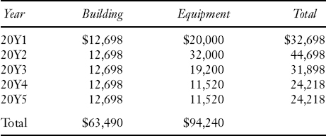
The Williams 5 & 10 extends no credit on its sales and pays for all its purchases immediately. The projections for sales and expenses for the new store for the next five years are:

The increase in inventory is an investment of cash when the store is opened, a $50,000 cash outflow. That is, management has to invest to maintain inventory while the store is in operation. When the store is closed in five years, there is no need to keep this increased level of inventory. If we assume that the inventory at the end of the fifth year can be sold for $50,000, that amount will be a cash inflow at that time. Since this is a change in working capital for the duration of the project, we include this cash flow as part of the asset acquisition (initially) and its disposition (at the end of the fifth year).

The tax basis of the building and equipment at the end of the fifth year are:

Tax basis of building = $400,000 − $63,490 = $336,510

and

Tax basis of equipment = $100,000 − $94,240 = $5,760

TABLE 26.1 WORKSHEET FOR THE WILLIAM 5 & 10 EXPANSION PROJECT

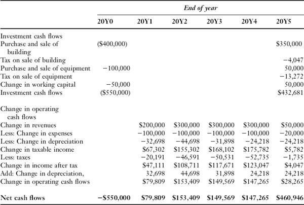
Since management expects to sell the building for $350,000 and the equipment for $50,000 after five years, the sale of the building brings a cash inflow of $350,000 at the end of the fifth year. The building is expected to be sold for more than its tax basis, creating a taxable gain of $350,000 − $336,510 = $13,490. The tax on this gain is $4,047. The sale of the equipment generates a cash inflow of $50,000. The gain on the sale of the equipment is $50,000 − $5,760 = $44,240. The tax on this gain is 30% of $44,240, or $3,272.

The pieces of this cash flow puzzle are assembled in Table 26.1, which identifies the cash inflows and outflows for each year, with acquisition and disposition cash flows at the top and operating cash flows below.

Now let's vary the assumptions. Suppose that the tax rate is not known with certainty, but may be any one of 20%, 30%, or 40%. The tax rate that we assume affects all the following factors:

• The expected tax on the sale of the building and equipment in the last year;
• The cash outflow for taxes from the change in revenues and expenses; and
• The cash inflow from the depreciation tax-shield.

Each different tax assumption changes the project's cash flows as follows:

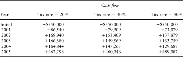
We can see that the value of this project, and hence any decision based on this value, is sensitive to what we assume will be the tax rate.

We could take each of the “what if” tax rate assumptions and recalculate the value of the project in terms of NPV. The impact on the NPV is shown below assuming a cost of capital of 5%:

Tax rate	NPV
20%	$331,134
30%	$276,679
40%	$249,954

But when we do this, we have to be careful because the NPV requires discounting the cash flows at a rate that reflects risk, and that is what we are trying to figure out! So we shouldn't be using the NPV method in evaluating a project's risk in our sensitivity analysis. An alternative is to recalculate the internal rate of return (IRR) under each “what if” scenario as shown below:

Tax rate	IRR
20%	20.20%
30%	17.77%
40%	16.32%

And this illustrates one of the attractions of using the IRR to evaluate projects. Despite its drawbacks in the case of mutually exclusive projects and in capital rationing, as pointed out in Chapter 6, the IRR is more suitable for use in assessing a project's attractiveness under different scenarios and, hence, that project's risk. This is because the NPV method requires management to use a cost of capital to arrive at a project's value, but the required return or cost of capital is what we set out to determine! Management would be caught in a vicious circle if it used the NPV method in sensitivity analysis. But the IRR method does not require a cost of capital or required return; instead, management can look at the possible IRRs of a project and use that information to measure a project's risk.

If we can specify the objective probability distribution for tax rates, we can put sensitivity analysis together with well-known statistical measures of risk. Suppose that in the analysis of the project management determines that it is most likely that tax rates will be 30%, although there is a slight probability that tax rates will be lowered and a chance that tax rates will be increased. Suppose further that the market is risk-neutral, in which case objective probabilities and risk-neutral probabilities coincide. More specifically, the table shows the probability distribution of future tax rates and the resulting IRR for the project:

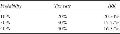
From the above distribution, it can be determined that the expected value for the IRR for this project is 17.433% and the standard deviation is 1.148%. Management could then judge whether the project's expected return is sufficient considering its risk (as measured by the standard deviation).

Management could also use these statistical measures to compare this project with other projects. However, although there is a measure of how widely dispersed the possible outcomes are from the expected value, it does not allow a comparison of standard deviations of different projects’ cash flows if they have different expected values. This is because comparing their standard deviations is meaningless without somehow adjusting for the scale of cash flows. Management can make comparisons by using a statistical measure known as the coefficient of variation. This measure translates the standard deviation of different probability distributions (because their scales differ) so that they can be compared. The coefficient of variation for a probability distribution is the ratio of its standard deviation to its expected value.

As can be seen from this illustration, sensitivity analysis allows management to assess the effects of changes in assumptions. But, because sensitivity analysis focuses only on one change at a time, it is not very realistic. We know that not one, but many factors can change throughout a project's life. In the case of the project considered by the management of Williams 5 & 10, there are a number of assumptions built into the analysis that are random variables, including the sales prices of the building and equipment in five years and the entrance of competitors no sooner than five years, to name only two.

26.3.2 Simulation Analysis

Sensitivity analysis becomes unmanageable if we change several factors at the same time. A manageable approach to changing two or more factors at the same time is simulation. Simulation analysis allows management to develop a probability distribution of possible outcomes, given a probability distribution for each variable that may change.

Suppose, for example, management is analyzing a project having the following three random variables: sales (number of units and price), costs, and tax rate. Suppose further that the initial outlay for the project is known with certainty and so is the rate of depreciation. From the firm's marketing research, management estimates a probability distribution for dollar sales. And from the firm's engineers and production staff and purchasing agents, management estimates the probability distribution for costs, which depends, in part, on the number of units sold. The firm's economists estimate the probability distribution of possible tax rates.

Management then has three probability distributions to work with. Now management needs a simulation model that can:

• Randomly select a possible value of unit sales for each year, given the probability distribution
• Randomly select a possible value of costs for each year, given the unit sales and the probability distribution of costs
• Randomly select a tax rate for each year, given the probability distribution of tax rates

Computers can be programmed to randomly select values based on whatever probability distribution is provided by management. Once the computer selects the number of units sold, the cost per unit, and the tax rate, the cash flows are calculated, as well as its IRR. Management now has one IRR or what is referred to as a “trial.” Then the computer starts all over by repeating this process, calculating an IRR each time. After a large number of trials, management will have a frequency distribution for the IRRs. A frequency distribution is a description of the number of trials the computer arrived at each different IRR value. Using the frequency distribution, management can calculate the expected value, the standard deviation, and coefficient of variation of the IRRs.⁵

To illustrate, let's use a simulation taken from Fabozzi and Peterson (2002). Suppose that management is considering the acquisition of $80 million in equipment for a new product. Through research with the marketing and production management, management has determined the expected price and cost per unit, as well as the number of units to produce and sell. Along with these estimates, management has developed standard deviations from past experience that provide information on the risk associated with these estimates. For simplicity, assume that these three random variables—price, cost, and number of units—are distributed normally with the means and standard deviations as estimated by management. The company's accounting department has provided an estimate of the range of possible tax rates during the product's life; in this example, a uniform distribution for these rates is assumed. This analysis has produced the following:

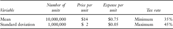
FIGURE 26.1 HISTOGRAM FOR SIMULATION ILLUSTRATION

Assuming that the product will be produced and sold for the foreseeable future and using Microsoft Excel, 1,000 draws were simulated (i.e., 1,000 random selections from each of the four variables’ distributions) using the above information. The new product's IRR is calculated for each of these draws, resulting in 1,000 IRRs or trials. The result is a distribution of possible IRRs, which are shown in the histogram in Figure 26.1. The height of this distribution is the number of draws (out of the possible 1,000 trials) for which the IRR fell into the range of IRRs depicted on the horizontal axis. In terms of risk, the wider the dispersion of possible IRRs relative to the expected IRR, the greater the new product's risk.

Simulation analysis is more realistic than sensitivity analysis because it introduces risk for many variables in the analysis. But this analysis may become complex since there are many interdependencies, both among variables in a given year and among the variables in different time periods. However, simulation analysis looks at a project in isolation, focusing instead on a single project's total risk. And simulation also ignores the effects of diversification for the owners’ personal portfolio. If owners hold diversified portfolios, then their concern is how a project affects their portfolio's risk, not the project's total risk.

26.4 MEASURING A PROJECT'S MARKET RISK

If management is looking at an investment in another firm, it could compare the potential acquisition's stock returns and the returns of the market over the same period of time as a way of measuring that stock's market risk. While this is not a perfect measurement, it at least provides management with an estimate of the sensitivity of that particular stock's returns as compared to the returns of the market. But what if management is evaluating the market risk of a new product it is considering introducing? Management cannot look at how that new product has affected the stock return of its own firm! So what does management do in such situtations?

26.4.1 Market Risk and Financial Leverage

Though management cannot look at a new project's returns and see how they relate to the returns on the market, management may be able to do the next best thing: estimate the market risk of the stock of another firm whose only line of business is the same as the project's. If management could identify such a company, it could look at the stock market risk of that company and use that as a first step in estimating the project's market risk.

Based on the CAPM, we will let β represent market risk. As the reader will recall from Chapter 14, β is a measure of the sensitivity of an asset's returns to change in the returns of the market. To distinguish the beta of an asset from the beta used for a firm's stock, we refer to an asset's beta as β_asset and the beta of a firm's stock as βequity. If a firm has no debt, the market risk of its common stock is the same as the market risk of its assets, and for that firm β_equity equals β_asset.

Financial leverage is created by the use of fixed payment obligations, such as notes or bonds, to finance a firm's assets. As we demonstrated in Chapter 5, the greater the use of debt obligations, the more financial leverage and the greater the risk associated with cash flows to owners. So the effect of using debt is to increase the risk of the firm's equity. If the firm has debt obligations, the market risk of its common stock is greater than its assets’ risk (i.e., β_equity > β_asset), due to financial leverage. Let's see why.

For any given firm, β_asset depends on the asset's risk, but not on how the firm chooses to finance it. As we have already mentioned, if management finances the firm with equity only, β_asset = β_equity. But what if management chooses to finance the firm partly with debt and partly with equity? Then the creditors and the owners share the risk of the assets, but because of the nature of the claims, not equally. Creditors have seniority and receive a fixed amount (interest and principal), so there is less risk associated with a dollar of debt financing than a dollar of equity financing of the same asset: The market risk borne by the creditors differs from the market risk borne by owners.

Representing the market risk of creditors as β_debt and the market risk of owners as β_equity, the asset's market risk is the weighted average of β_debt and β_equity. If the proportion of the firm's capital from creditors is ω_debt and the proportion of the firm's capital from owners is w_equity, then: ⁶

or

β_asset = β_debt w_debt + β_equity w_equity

But interest on debt is deducted to arrive at taxable income, so the claim that creditors have on the firm's assets does not cost the firm the full amount, but rather the after-tax claim, so the burden of debt financing is actually less due to interest deductibility. Further, the beta of debt is generally assumed to be zero (i.e., there is no market risk associated with debt). With D representing the market value of debt, E representing the market value of equity, and τ the marginal tax rate, the relation between the asset beta and the equity beta is:

This means that an asset's beta is related to the firm's equity beta, with adjustments for financial leverage. If a firm does not use debt, β_equity = β_asset and if the company does use debt, β_equity > β_asset.

Therefore, β_equity may be translated into β_asset by removing the influence of the firm's financial risk. To accomplish this, the following must be known:

• The firm's marginal tax rate
• The amount of the firm's debt financing in market value terms
• The amount of the firm's equity financing in market value terms

The process of translation is referred to as “unlevering” because the effects of financial leverage are removed from the equity beta, β_equity, to arrive at a beta for the firm's assets, β_asset. This therefore is an estimate of the market risk of a firm's assets.

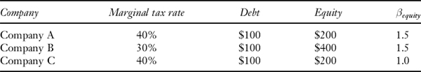
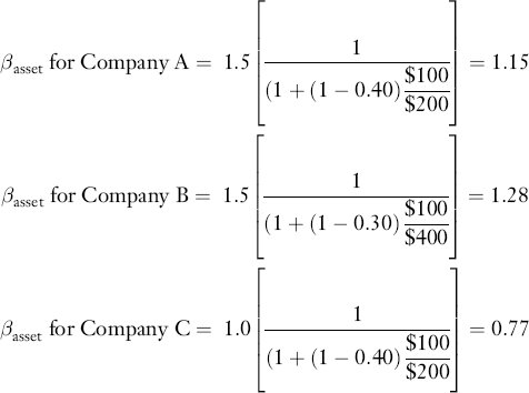
To illustrate the unlevering of the equity beta, consider the following three companies:

Then,

26.4.2 Using a Pure-Play Firm

There are many instances in which management invests in assets with differing risks and is therefore faced with estimating the cost of capital of a project. Using the firm's asset beta would not be appropriate because the asset beta reflects the market risk of all of the company's assets and this may not reflect the risk of the project being evaluated. One approach to dealing with this dilemma is to estimate the cost of capital for a company with a single line of business similar to the project under consideration. Such a company is referred to as a pure-play firm.

One method of estimating the pure-play firm's equity beta is to regress the pure-play firm's stock returns against the returns on the market portfolio. Once the pure-play firm's equity beta is calculated, management then “unlevers” it by adjusting it for the financial leverage of the pure-play firm.

Examples of pure-play equity betas in 1994 are shown in Table 26.2. The firms listed in this table have one primary line of business. Using the information for Alcan Aluminum and assuming a marginal tax rate of 35%, we see that the asset beta for aluminum products is 0.748:

A firm such as Gap, Inc. with little debt relative to equity will have an asset beta that is close to its equity beta.

TABLE 26.2 EQUITY AND ASSET BETAS FOR SELECTED FIRMS WITH A SINGLE LINE OF BUSINESS

Note: The book value of debt is used in place of the market value of debt since the latter is not readily available. The market value of equity is the product of the number of shares outstanding and the closing share prices as of the end of the year. A 35% tax rate is assumed.

If an appropriate pure-play firm can be identified, this method can be used in estimating a project's cost of capital.⁷ However, since many U.S. corporations have more than one line of business, finding an appropriate pure-play firm may be difficult. Care must be taken by management to identify firms whose lines of business are similar to the project's.

26.4.3 Adjusted Present Value

The use of the project's cost of capital to discount the cash flows of a project to the present is one method of incorporating the effect of financial leverage into the evaluation of a project. Another method is the adjusted present value (APV) method, which involves separating the value of the project's leverage from the value of the project itself.⁸ In other words,

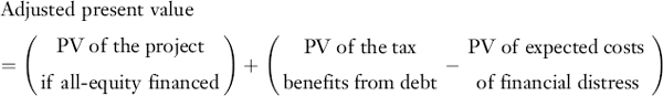
The value of the project if all-equity financed is the present value of the project's cash flows, discounted at the asset beta, β_asset.

The value of the tax benefits from debt is the present value of the tax-shield from interest deductibility. Using the company's capital structure as a measure of the anticipated debt financing relevant to consider for this project and indicating the marginal tax rate as τ, the after-tax cost of debt as r_d^* and the amount of debt as D, the present value of the tax shields is: ⁹

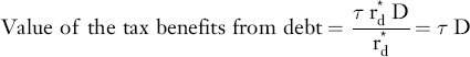
If we assume that the company finances its projects similar to its target debt-equity ratio, D/E, then:¹⁰

The present value of the expected costs of financial distress is the present value of the probability-weighted costs of bankruptcy:

Suppose management is evaluating a project that has a required initial outlay of $6 million and expected cash flows of $1 million per year for each of the next 10 years. And suppose that the marginal tax rate is 35%, the company's capital structure has a D/E ratio of 60%, an after-tax cost of debt of 3.25%, and a cost of equity of 8%. The cost of equity is estimated by using the company's beta of 1.5, an expected risk-free rate of interest of 3%, and an expected return on the market of 6.4%. In the traditional NPV method, the project's cost of capital is:

Project cost of capital = (0.375)(0.0325) + (0.625)(0.08) = 6.2188%

and the value of the project is $1.2844 million.

Using the APV method, it is first necessary to unlever the equity beta to remove the effects of leverage:

Therefore, the cost of equity is:

r_e = 0.03 + 1.21(0.064 − 0.03) = 0.03 + 0.04114 = 0.07114 or 7.114%

The value of the all-equity financed project is therefore $0.9867 million.

The debt for the project is the project cost, $6 million, multiplied by the debt-asset ratio:

The present value of the tax shields from debt are:

Value of the tax benefits from debt = (0.35)$2.25 = $0.7875

Without considering the effect of financial distress, the APV is:

APV = $0.9867 + 0.7875 = $1.7742

The challenge is therefore to incorporate the cost of financial distress. If it is assumed that there is a 10% chance the company could experience financial distress and that financial distress would result in a loss of 100% of the project's value, the present value of the costs of financial distress are:

PV of the costs of financial distress = (0.10)($0:9867) = $0.09867

The APV considering the effect of financial distress is therefore:

APV = $0.9867 + 0.7875 0.09867 = $1.6558

The NPV and APV methods produce different values for the project: $1.2844 versus $1.6558.¹¹ This is typically the case in comparing the two methods because the NPV method incorporates the benefit of taxes and the costs of financial distress in the project's cost of capital, whereas the APV adjusts for these separately.

What are the advantages of using the APV approach? In the traditional method the effects of the tax deductibility of interest and of financial distress are reflected in the costs of capital. The APV segregates those effects, thus requiring mangement to focus specifically on incorporating both the probability and the costs of financial distress.¹² The APV method also allows for more flexibility in specifying the debt level anticipated in the future.

26.5 CONTINGENCY PLANNING OF CAPITAL EXPENDITURES

In our Chapter 10 discussion of contingent claims and contingent strategies we explained how management decisions can differ in different states of the world, and how payoffs may be improved by making decisions that are contingent on the currently prevailing state of the world. We also explained how contingent strategies provide ways to manage risks and information about them.¹³

Chapter 10 provided an example of a contingency strategy for a firm planning to select a location and build a factory that might later be expanded. In this section, we provide a second example in which contingency planning can commit the firm to successive stages of an investment program as more information is gleaned regarding the proposed project.¹⁴ We assume for simplicity that the particular decision can be assessed separately from others the firm will take and that management uses expected present value maximization as a criterion function. We shall later illustrate how to take risk into account as well.

26.5.1 Example

Here is the setup for the example. The Perils of Pauline Cereals, Inc. has recently developed a new product. Pauline Cereals is now attempting to determine whether marketing the product would be a financially sound decision and, if so, what type of marketing strategy should be employed.

Introduction of the new product would require an initial cash outlay of $725,000 to prepare a production setup with a useful producing life of about one year. The production setup would have a capacity great enough to meet the production requirements of any of the possible plans for product introduction that marketing has developed. Apart from initial cash requirements, discrepancies between revenue and cash flows during the year can be financed at short-term rates, the costs of which are included in the estimates we shall give. The $725,000 is not recoverable if plans are later cancelled; as an alternative these funds could be invested in another project almost certain to yield 7%.

The Marketing Department has prepared a variety of plans for different marketing conditions. These involve either the initial introduction of the product on a national scale or a plan for test marketing, following the results of which a decision to terminate the sales effort or to distribute the product nationally can be made. If the test market plan is followed, there is a possibility that a competitor's product will appear and cut into sales. Furthermore, the probability of competition appearing is increased if the test marketing plan is successful. However, because of the timing involved, immediate national distribution would rule out the possibility of competition.

Marketing has prepared certain estimates of market conditions and the probability of a competitor's product appearing. The Marketing Department believes that the probability a test marketing campaign will be successful¹⁵ is about 0.5. If the test market campaign is successful, Marketing judges that the probability of a competing product appearing is 0.8, but if the test marketing campaign is unsuccessful, the probability of a competing product appearing is only 0.4.

TABLE 26.3 STRATEGIES’ PAYOFFS AND PROBABILITIES

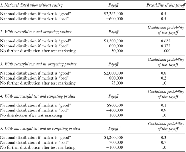
The Controller's Division, working with the Marketing Department, has prepared the estimates of payoffs from the different plans as shown in the first panel of Table 26.3. The payoffs are realized after the expenditure of $725,000 and take into account the fact that the national market can (without testing) be characterized as being either a “good” market or a “bad” one. Each payoff is expressed in terms of a lump sum available one year from now and includes all costs and revenue (including any necessary short-term financing) except for the initial $725,000.

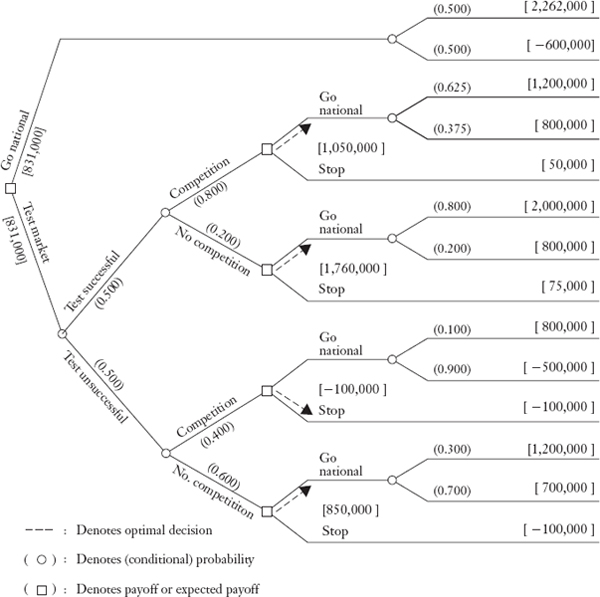
FIGURE 26.2 DECISION TREE FOR PERILS OF PAULINE PROBLEM

Similarly, the Controller's Division has prepared the various forecasts of the realizable payoffs after test marketing strategies have been followed and their outcomes ascertained. These payoffs are shown in the the panels in Table 26.3. Once again, the Controller's Division has found it convenient to classify post-test market strategies as either “good” or “bad.” However, these conditions (and hence their payoffs) are not directly related to those forecast without test marketing, because the test marketing approach itself, being a learning experience, has an effect on payoffs that can subsequently be earned.

What plan of action should the management follow? Why?

The Perils of Pauline problem can be structured in the form of a decision tree as shown in Figure 26.2. The important characteristics of such a tree are that all possible choices of the decision maker, as well as all possible outcomes of the random variables, are displayed in their logical order as branches of the tree. Note that events are depicted in their natural sequence and that distinctions are made between branches which can be selected by the decision maker, and branches which are selected through the realization of a random variable. The branches at which choices can be made by the decision maker are indicated by nodes with rectangular boxes drawn around them. The dollar payoffs from decision-outcome sequences are recorded at the ends of the branches. Note how the tree displays the notion of contingent strategies as a part of its logic. For example, the second upward-pointing branch of the tree shows that even if the test marketing strategy is successful, management need not commit the firm to a national distribution decision until after it has been determined whether or not a competitor will enter the market.

The solution technique for finding the best contingent strategy involves working backward through the tree, writing down at each decision node the payoff to be earned by following the best branch of the tree from that point on, and using that information in calculations for earlier points in time.¹⁶

To see the logic of the solution technique, consider the second branch from the upper side of the tree in Figure 26.2, depicting the decisions either to introduce the product nationally or to stop. If the company were on the lower twig of this branch, the expected value of going national would be:

0.8($2,000,000) + 0.2($200,000) = $1,640,000

while the expected value of stopping would be $75,000. Clearly, if the management finds itself in this situation, the best way to continue is by introducing the product nationally, as is shown by the arrow and the value of $1,640,000 in brackets.

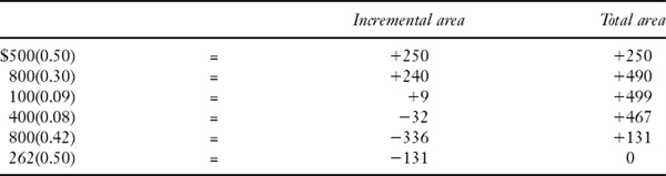
The same calculations are made for each possible decision point at which the firm could arrive when the second decision must be made, and they are then carried backwards in time to the decisions, which, if initially taken, could have placed the company in that position. Thus, for example, the four decision points that could be reached by following a test market strategy are shown in the lower half of the tree and have (at the time one of these four decisions must be taken) the values $1,050,000, $1,640,000, $100,000, and $850,000. Multiplying these values by the conditional probabilities of their occurring, the expected payoff from the test market strategy is seen to be:

In Figure 26.2 the best decisions are indicated by the arrows. The two best strategies in terms of expected value, as calculated from the tree, are given in Table 26.4 along with their payoff distributions. The fact that the two uncertain payoffs have identical expected values reflects the contrived nature of the example and will be used for further discussion shortly. Note, however, that the immediate national distribution strategy is actually a noncontingent strategy in that it merely prescribes acting on the basis of the most likely outcome when no test marketing is conducted.

TABLE 26.4 DISTRIBUTION OF PAYOFFS FOR STRATEGIES A AND B

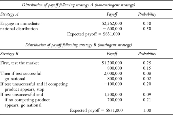
In this example the advantage of the test marketing (contingent) strategy is not a higher expected payoff but rather the lower risk with which that payoff is earned. Indeed, the equality of expected payoffs in the example was designed to emphasize the point that expected values may not capture all relevant aspects of probabilistic payoffs if the decision maker is risk averse. Formally, of course, the difficulty is dealt with by assuming utility functions that are additive or multiplicative in different periods’ payoffs and using dynamic programming or other routines to compute expected utility. However, it is sometimes possible to rank probabilistic payoffs using only the knowledge that the decision maker is risk averse. As explained next, the method of stochastic dominance, which performs such rankings, is useful in problems that have only terminal payoffs.¹⁷

26.5.2 Application of Stochastic Dominance

To see how the concept of stochastic dominance is relevant to the example, recall that we showed in Chapter 12 how two probability distributions may be ordered by second degree dominance for any risk-averse decision maker.¹⁸ Using the results of Chapter 12, we find that the payoffs earned from following strategy B would be preferred to those earned from following strategy A by every risk-averse decision maker.

FIGURE 26.3 CUMULATIVE DISTRIBUTIONS OF PAYOFFS FROM STRATEGIES A AND B

TABLE 26.5 STOCHASTIC DOMINANCE CALCULATIONS FOR STRATEGIES A AND B (VALUES EXPRESSED IN HUNDREDS OF THOUSANDS)

The stochastic dominance calculations comparing A and B are given in Figure 26.3 and Table 26.5. Strategy B and the certain alternative, C, cannot be compared using stochastic dominance because in the latter case the criterion exhibits a sign change. Thus, even though alternative A can be eliminated because it is in effect riskier than alternative B, two alternatives still remain. Either B or C should be selected by a given decision maker on the basis of a more closely specified attitude toward risk.

26.6 REAL OPTIONS VALUATION

Using a decision tree to analyze a risky project provides one example of real options valuation (ROV). The option in the previous example is to expand in stages if the test marketing strategy is successful.¹⁹ Consider other typical options inherent in an investment opportunity:

• Most every project has an option to abandon, though there may be constraints (e.g., legally binding contracts) that affect when this option can be exercised.
• Many projects have the option to expand.
• Many projects have an option to defer investment, putting off the major investment outlays to some future date.

So how should we analyze these options? As our example has already shown, one approach is to use decision tree analysis, associating probabilities to each of the possible outcomes for an event and mapping out the possible outcomes and the value of the investment opportunity associated with these different outcomes. While this approach is workable when there are few options associated with a project, option pricing theory offers a method of analysis that provides additional useful information.

The basic idea of ROV is to recognize that the value of a project extends beyond its value as measured by a noncontingent calculation of NPV; in other words, the value of project is supplemented by the value of the contingent strategies represented as options. Since options are considered to be strategic decisions, the NPV based on contingency strategies is often referred to as strategic NPV. Consider an investment opportunity that has one option associated with it. The strategic NPV is the sum of the traditional NPV—referred to as the noncontingent NPV or static NPV—and the value of the option:

Strategic NPV = Noncontingent NPV + Value of the option

26.6.1 Options on Real Assets

The valuation of options is simple in concept, as both Chapter 19 and the Perils of Pauline example have already illustrated. However, although the underlying concepts are the same as those already illustrated, it may appear substantially more complex to apply traditional forms of option pricing theory, such as the Black-Scholes model (1973). The Black-Scholes model is based on five factors that have been shown to be important in valuing an option:

1. The value of the underlying asset, P
2. The exercise price or strike price of the option, E
3. The risk-free rate of interest, r
4. The volatility of the value of the underlying asset, σ
5. The time remaining to the expiration of the option, T

TABLE 26.6 RELATION BETWEEN THE FACTORS THAT AFFECT THE VALUE OF A STOCK OPTION AND THOSE THAT AFFECT A REAL OPTION

Source: Fabozzi and Peterson (2002).

In Chapter 19, we examined the relation between each of these factors and the value of a stock option. Our focus here is to map these factors into a real option setting. Like other options, real options can be calls (options to buy assets), puts (options to sell assets), or compound options (options on other options). And, like other forms of option instruments, real options may be European (capable of exercise only on the expiration date) or American (capable of exercise at any time on or before the expiration date).

In general terms, the relation between the factors that affect the value of a stock option and those that affect a real option correspond as shown in Table 26.6. Of course, the factors that correspond to a specific option can be better described when we examine the particular option. Consider the option to abandon. In this case, the underlying asset is the value of continuing operations. The strike or exercise price for this option is the exit value or salvage value of the asset. A number of common real options are described in Table 26.7.

TABLE 26.7 EXAMPLES OF REAL OPTIONS

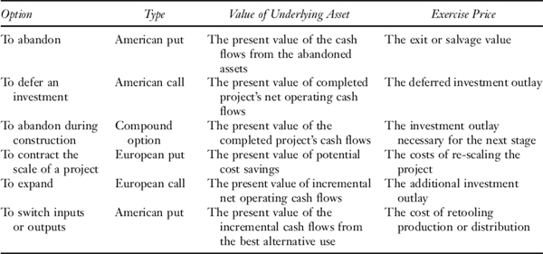
Source: Fabozzi and Peterson (2002).

Identifying the options associated with an investment opportunity is the first step. The second step is to value these options. Consider an investment opportunity to defer an investment. This investment opportunity is similar to what a firm experiences in their investment in research and development (R&D): an expenditure or series of expenditures are made in R&D, and then sometime in the future depending on the results of the research and development, the actions of competitors, and the approval of any regulators, the firm can then decide whether to go ahead with the investment opportunity.

26.6.2 Real Options: An Example

Let's put some numbers to the analysis of this project using an illustration from Fabozzi and Peterson (2002). Suppose that research and development is expected to cost $2.5 million for each of the first four years. And suppose that at the end of the fifth year the firm has an option to either go ahead with the product or simply abandon it. If the firm goes ahead with development of the product, this will require an investment of $80 million at the end of the fifth year. To make the analysis simpler, let's assume that we can sell the investment in the product—that is, cash out—at the end of the fifth year for $100 million.²⁰

Using a discount rate of 20% (continuously compounded), the NPV of this investment opportunity is $1.36 million as shown below:²¹

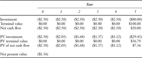
Using traditional capital budgeting, the foregoing analysis suggests that we should reject the project because its NPV is less than zero. But we have not yet considered the valuable option of the deferred investment. Management can wait until the end of the fifth year to decide whether it wants to commit the additional $80 million. Meanwhile, management invests in the R&D in each of the first four years.

So how much is this option worth? We need to make a couple of assumptions regarding the risk-free rate of interest and volatility. Suppose that the risk-free rate of interest is 5%, the market risk premium is 6%, and the volatility (i.e., the standard deviation of the project's cash flows) is 2.5 times that of the market volatility. Since the market volatility is 20%, the option volatility is 50%. The cost of capital is calculated as follows using the risk-free rate and the market risk premium is 20%:

Cost of capital = 5% + 6%(50%/20%) = 5% + 15% = 20%

The value of the factors that are considered in the option valuation are then as follows:

Parameter	Value
Value of underlying asset	$36.79 million
Exercise price	$80 million
Risk-free rate of interest	5%
Volatility	50%
Number of periods to exercise	5 years

The value of the underlying asset is the present value of the additional outlays needed to go ahead with the project, discounted at a continuously compounded rate of 20%:

Value of underlying asset = $100 million e^−.20(5) = $36.79 million

Using the Black-Scholes option pricing formula,²² the value of this option is $10.24 million. Does this change the decision of whether to invest? The strategic NPV is:

Strategic NPV = Static NPV + value of the option

Strategic NPV = −$1:36 million + $10:24 million

Strategic NPV = $8:88 million

Hence, the project has a positive NPV considering the valuable option that is associated with it.

26.6.3 Challenges in Implementing ROV

We used a straightforward example to illustrate the importance of considering options. Now let's examine a couple of the challenges in incorporating ROV into an actual investment opportunity analysis.²³

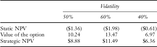
The first challenge has to do with the parameters of the model. Focusing just on the estimate of volatility, we can see that the value added of the option is sensitive to the estimate of volatility. Though we simply assumed that the volatility is 50%, it is not a simple matter to determine the volatility of a project's future cash flow. We experience the same problems that we did in trying to determine the beta of a project—it just isn't measurable directly. The volatility of an investment opportunity's cash flows affects two key elements of the strategic value: (1) the volatility has a positive relation to the value of the option (i.e., the greater the volatility, the greater the value of the option), and (2) the volatility has a negative relation to the static NPV (i.e., the greater the volatility, the greater the cost of capital, and hence the lower the static NPV). If we take this last example and calculate the strategic NPV with volatility of 60% and 40%, as well, we see that the value of the option is affected by the choice of volatility:

Second, most investment projects have several options, and some of them interact. For example, if a firm is investing in R&D over a period of years in the development of a new product, there exists at least two options: the option to abandon during development and the option to defer investment. The valuation problem in the case of multiple options is not simply carried out by adding the separate values because the value of one option may affect the value of other options. Solving for the value of options in the case of multiple, interacting options can be quite difficult, requiring the application of numerical methods.²⁴

KEY POINTS

• To evaluate the riskiness of a project, management must begin by recognizing that the assets of a firm are the result of its prior investment decisions and hence, that the firm is a portfolio of projects.
• Although management should consider how a given project increases asset portfolio risk, in practice, management typically focuses on measuring the stand-alone risk of the individual project.
• One approach to evaluating a risky project is to use a risk-adjusted discount rate.
• Within the risk-adjusted discount rate approach, a commonly used method for estimating a project's cost of capital or market-required rate of return is to use the CAPM. That requires specifying the premium for bearing the average amount of risk for the market as a whole and then, using a measure of market risk, fine-tuning this to reflect the project's risk.
• Because in practice it is not simple to estimate a project's beta, an alternative is for management to begin with the weighted-average cost of capital and adjust it based on the project's perceived risk.
• The certainty-equivalent approach is an alternative to the risk-adjusted discount rate. Using risk-neutral probabilities is one way to calculate a project's market value—a particular form of certainty-equivalent value.
• A project's total risk or stand-alone risk can be estimated based on the objective probability distribution for the risky cash flows. It is a project's market risk that is relevant to the management in making a capital budgeting decision.
• A project's beta risk can be estimated by looking at the market risk of firms in a single line of business similar to that of the project, a pure-play.
• An alternative to finding a pure-play is to classify projects according to the type of project (e.g., expansion) and assign costs of capital to each project type according to subjective judgment of risk.
• Sensitivity analysis and simulation analysis are tools that can be used in conjunction with statistical measures to evaluate a project's risk. Both techniques give us an idea of the relation between a project's return and its risk.
• Contingent strategies provide an alternative framework to evaluate risky projects.
• The real options valuation approach involves estimating the options associated with an investment opportunity and helps management identify value in a project that is not reflected using traditional capital budgeting techniques. Real options can be valued using either decision trees or option pricing formulae.
• There are options associated with every investment opportunity, including the option to defer the investment and the option to abandon the investment.
• The valuation of a single option is straightforward but the valuation of multiple options, especially if they interact, can be quite difficult.

QUESTIONS

1. What is the difference between sensitivity analysis and simulation analysis?
2. Why is the internal return method a better method to employ in capital budgeting analysis than the net present value method when evaluating/assessing a project's attractiveness under different scenarios?
3. a. What are the difference between net present value and the adjusted present approaches?

   b. What are the advantages of using the APV approach?

4. The XYZ Company has a financial structure that includes debt and equity. There is no preferred stock in the capital structure. The portion of the capital structure financed by debt is 55%. Management estimates that the beta of the debt is 0.3 and the beta of the total assets is 0.5. What is the beta of XYZ Company's equity?
5. What is the relationship between the volatility of an investment opportunity's cash flows with its static net present value and value of the option?
6. Suppose the beta of a firm's assets is k and the tax rate is 40%. What is the debt-to-equity ratio if the beta of the equity is 4 times the beta of the assets?
7. Suppose management of Company ABC is evaluating a project which has an initial outlay of $10 million and an expected cash flow of $3 million per year for each of the next five years. Assume that the company's (i) marginal tax rate is 40%, (ii) debt-to-equity ratio equal to 1, and (iii) after-tax cost of debt of 4% and a cost of equity of 6%. The cost of equity is estimated using the Capital Asset Pricing Model assuming a beta of 1.2, a risk-free interest rate of 3%, and an expected return on the market of 7%.
   1. What is the net present value for this project?
   2. What is the adjusted present value for this project if the effect of financial distress is ignored?
8. Consider once again the information in question 7 and now consider the cost of financial distress. Assume that management believes there is 20% and 30% chance that financial distress would result in a loss of 80% and 40%, respectively, of the project's value. Recalculate the adjusted present value of the project.
9. Suppose that a project costs $1 million for each of the first five years. At the end of the fifth year, the firm can either abandon the project or continue to operate it. If the project is continued, the expected payoff is $6 million as of the end of the end of the fifth year applying the Black-Scholes option pricing model. For the value of this option to abandon or continue is $3 million. What is the strategic net present value of this project if the cost of capital is 5%?
10. Management is considering entering into a contract to produce a product. The product will be sold at the end of second year for a price of $8. Below is the cash flow of a product under consideration by management. At the end of the second year, management has the option to abandon the project or continue with the development of the project for another investment of $6 million at the end of the second year.

    

    If the cost of the capital is 15% by continuous compounding, the risk-free rate is 5% and the volatility is 0.3. What is the Static NPV and what is the Strategic NPV?

REFERENCES

Amram, Martha, and Nalin Kulatilaka. (1999). Real Options. Boston: Harvard Business School Press.

Black, Fischer, and Myron Scholes. (1973). “The Pricing of Options and Corporate Liabilities,” Journal of Political Economy 81: 637–659.

Fabozzi, Frank J. and Pamela P. Peterson. (2002). Financial Management and Analysis. Hoboken, NJ: John Wiley & Sons.

Hull, John. (2003). Options, Futures, and Other Derivatives (5th ed.). Upper Saddle River, NJ: Pearson.

Moore, William. (2001). Real Options and Option-Embedded Securities. Hoboken, NJ: Wiley.

Myers, Stewart C. (1974). “Interactions in Corporate Financing and Investment Decisions—Implications for Capital Budgeting,” Journal of Finance 29: 1–25.

Myers, Stewart C. (1977). “Determinants of Corporate Borrowings,” Journal of Financial Economics 5: 147–176.

Trigeorgis, Lenos. (1991). “A Log-Transformed Binomial Numerical Analysis Method for Valuing Complex Multi-Option Investments,” Journal of Financial and Quantitative Analysis 26: 309–326.

Trigeorgis, Lenos. (1993). “Real Options and Interactions with Financial Flexibility,” Financial