
20
CAPITAL MARKET IMPERFECTIONS AND FINANCIAL DECISION CRITERIA
In this chapter we recognize a variety of capital market imperfections and then outline their consequences for the financial theories we have so far developed. Capital market imperfections have a potential for creating important consequences for financial decision making. However, these consequences depend both on the nature and on the ubiquitousness of the imperfections. These are matters related more closely to applications than to theory and we will explore applications further in the book's remaining parts. But first it is useful to outline how the theory itself is changed by the phenomena we now recognize.
We shall argue that the major imperfection affecting financial market prices involves the collection and dissemination of information that seems often to be distributed quite unevenly. At the same time, auction markets like the stock exchanges are clearly efficient despite the presence of such imperfections as transactions costs. Thus, in the sequel we shall pay considerable attention to heterogeneously distributed information and less to issues involving explicit charges such as flotation and brokerage costs. We also argue, on occasion, that markets may be incomplete in the sense of Chapter 16, and the effects of incompleteness will, from time to time, augment the effects of heterogeneously distributed information.
20.1 TYPES OF CAPITAL MARKET IMPERFECTIONS
There are several kinds of capital market imperfections whose existence appears to be potentially important for explaining real-world financial decisions. We first categorize these imperfections, then investigate their importance.
20.1.1 Heterogeneous Expectations
In a risky world, differences of opinion regarding the probability distributions characterizing future events may arise. That is, investors may have heterogeneous expectations. Even if we assume all investors are privy to the same data regarding past events, they might form different probability distributions regarding possible future events. Accordingly we must consider the implications of possibly differing probability distributions, both for financial theory and for the decisions they prescribe.
We use the concept of a contingent claim discussed in Chapter 10 to develop the essence of the argument. We assume there are two possible future states of the world, and that our task is to assess the effects of a contingent claim's differing values under the following three sets of conditions:
| Condition 1. | Homogeneous expectations and risk neutrality. Assume that everyone agrees on the following data for the contingent claim and the associated objective probabilities:
Also, assume that the one-period risk-free rate is r. Then the time 1 value of the contingent claim, denoted by C (1) is: C(1)= [p(1)+(1 − p)(0)]/(1 + r) because risk-neutral investors capitalize the risky prospects’ expected values at the risk-free rate of interest. The assumption of investor agreement implies that the time 1 value will also be the market price of the claim. |
| Condition 2. | Homogeneous expectations, risk-averse investors. In a perfect capital market, we can estimate risk-neutral probabilities from market price data. In this case, the value of claim one can be calculated as:
C*(1) = [q(1) + (1 − q)(0)]/(1 + r) < C(1) assuming that the (estimated) risk-neutral probability q, p and1 that the risk-free rate is the same as before. Again, because of investor agreement, the value C* (1) will be the market price of the claim. But C*(1) < C (1), reflecting the risk premium demanded by the market. |
| Condition 3. | Heterogeneous expectations, risk-averse investors. We now assume each investor i attaches her own risk-neutral probability qi to state 1 and 1 − qi to state 2. We continue to suppose that all investors agree on the risk-free rate. Under these assumptions, the value of the contingent claim to investor i is:
and Ci*(1) may be either less than or greater than C*(1). That is, each investor's valuation of a contingent claim varies according to the subjective value of the risk-neutral probability she attaches to state 1. The time 1 market value of contingent claims then depends on the number of different investors, their demands for claims as implicitly defined by the foregoing equation, and the supply of claims. It is convenient to elaborate these effects on market value by using a more extended example. |

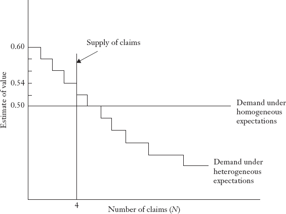
Let us now suppose that there are N contingent claims outstanding in the capital market and that each investor may buy at most one such claim. (The claim prices are now chosen for convenience and are not calculated from the data of the earlier example.) Each investor i will buy a claim if his or her valuation of claim Ci(1) is at least as great as the claim's market price, denoted Cm(1). Assuming N to be 4, we assume the data shown in Table 20.1, from which Figure 20.1 is drawn.2 Under the assumption that investors differ in their subjective estimates of risk-neutral probabilities, the stepped line of the figure indicates the demand function of all potential investors at various market prices for the contingent claims. Note that as the price of the contingent claims falls, more investors are willing to purchase a claim. The horizontal straight line shows the market demand function for the claims if all investors agree regarding their probability assessments. We show the two demand curves intersecting at the same price for the average investor. This means that when expectations differ, about as many investors attach a high value to the stock as the number attaching a low value. The vertical line at N = 4 represents the available supply when no short selling is permitted, and the market-clearing price is established by the intersection of the market supply and demand curves. When N is small relative to the number of potential investors, the market price will be higher than it is under homogeneous expectations, at least if enough of the investors are more optimistic than the average, as in our example.
TABLE 20.1 DATA FOR FIGURE 20.1
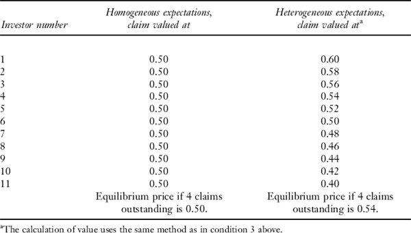
FIGURE 20.1 MARKET-CLEARING VALUE OF CONTINGENT CLAIM UNDER HETEROGENEOUS
The reasoning applied to contingent claims can be applied to any security. When it is applied to stocks, several conclusions follow from this model of heterogeneous expectations: 3
- As long as the entire supply of shares can be absorbed by a minority of the potential purchasers, the market-clearing price will be above the mean evaluation of the potential investors.
- Under condition 1, an increase in divergence of opinion4 will increase the market-clearing price, and a decrease will reduce the market-clearing price. (When the divergence of opinion decreases to the point where there is no disagreement, we are back to the case of homogeneous expectations.)
- If potential investors make unbiased estimates of the distribution of mean returns from possible investments and make investments on the risk-return basis of standard portfolio theory, the market-clearing price of shares will exceed the willingness to pay of an investor with perfect information about the probability distribution of returns.
- Under condition 3, if firms make their investment decisions to maximize the market value of their shares, there will be excess investment in those firms and industries about which there is the greatest divergence of opinion, and these may well be the riskier alternatives.
In the foregoing discussion we assumed the supply of securities to be small relative to the number of potential investors. This may not be so if markets are somehow segmented: For example, if large private placements are sold to a small number of institutional investors. In these contrary cases, heterogeneous expectations would lower rather than raise prices. This may be a partial explanation for why certain classes of firms, such as new ventures, frequently seem to have considerable difficulty raising finance capital.
In any event, with heterogeneous expectations our reliance on models like the contingent claims model (just mentioned) or like the CAPM is weakened, because a market equilibrium price is much less easily predicted. Unless we have more details about how opinion diverges, we cannot say whether price will be higher or lower than that predicted by a model like the CAPM. Nevertheless, we do not regard these statements as saying that our earlier theories should be abandoned. Rather, it seems that they may still provide approximately correct pictures of real-world conditions, at least for portfolios of stocks. Thus, if we wish to assume heterogeneous expectations, the task becomes one of assessing the degree of approximation involved in a given financial decision problem.
20.1.2 Unequally Distributed Information
The situation regarding risky future outcomes is actually more complex than a discussion of heterogeneous expectations suggests. For not only may investors have different expectations regarding the future, they may not even share the same information about the past. For example, a seller of fire insurance, knowing that a client has lodged a claim for fire damage, will not always be able to tell (at least for any reasonable cost) whether the client deliberately set the fire or not. Of course, the client has this information, but a dishonest client cannot be expected to admit culpability.
To give another example more closely related to financial management, an investor may not have the same information about either a firm's history or its prospects as does the firm itself. Moreover, the latter may not wish or perhaps even be able completely to convey available information.5 The last problem is especially important in cases where a public offering of securities is made. In these cases most legal jurisdictions have securities regulations stipulating that the company's plans be outlined in a prospectus. But there are well-known difficulties to incorporating all relevant information, especially that of a qualitative nature, in such a document. For these reasons, it may be difficult for potential investors to assess accurately the nature of the risks involved in purchasing the securities of some firms. Accordingly, potential investors may not all have the same data with which to make assessments of the firm's future, and even if they do, all investors may not assume the same probability distributions in describing a firm's prospects. A similar situation may obtain in negotiated markets where borrowers’ credit risks may be difficult to establish.6
20.1.3 Transactions Costs and Tax Differentials
If when making financial transactions an investor must pay charges other than interest rates (e.g., loan application charges, brokerage charges on stock sales), the ability to move along a wealth constraint of equal present values is impaired. In particular, any profile of cash flows different from that determined by income receipts may have a lower present value than that of the income receipts themselves, because the investor might have to pay transactions charges to make the conversion from one cash flow profile to another.
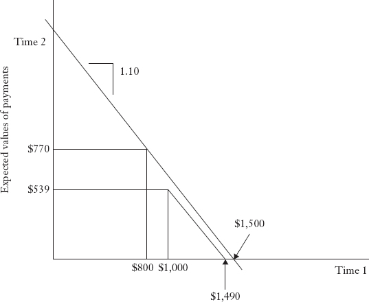
To see the effects of transactions charges, suppose that all investors are risk neutral, that an investor has an income stream with expected values of $800 and $770 at times 1 and 2, respectively, and that interest rates are 10%. Then the present value of this income stream is $1,500. Now suppose the investor wishes to spend $1,000 at time 1. In a perfect capital market this means the expenditure stream is ($1,000, $550), which also has a present value of $1,500. But if markets are imperfect in the sense that to borrow the $200 to finance time 1 consumption the investor must pay, in addition to interest charges, a commission having a time 1 value of $10, then the expenditure stream is $1,000 and $539) in times 1 and 2, respectively, with a present value of $1,490. Hence, the investor cannot move freely along the wealth constraint, shown as a solid line in Figure 20.2, but must instead accept a reduction in net present value to reallocate income in the fashion indicated. Hence, this investor is not indifferent between the income stream $800 and $770, and the income stream $1,000 and $550 (both for times 1 and 2, respectively) even though the streams both have the same net present value when transaction charges are not paid.
A similar conclusion applies to selling shares. An investor may prefer dividend income to realizing capital gains through share price appreciation, if in the latter case brokerage charges to sell shares must be paid. On the other hand, the problem is the same but the conclusions may be reversed with respect to the effects of taxation. If, for example, income taxes are levied but capital gains are taxed at a lower rate than ordinary income, investors will not be indifferent between dividend and share price increases; they may have a distinct preference for the latter.
For all the foregoing reasons, the separation of managers’ wealth-maximizing decisions from the consumption decisions of their firm's stockholders is no longer always possible. The implications of this are considered further in Section 20.3.
FIGURE 20.2 EFFECT OF TRANSACTIONS CHARGE ON THE WEALTH CONSTRAINT
20.1.4 Costs of Unsystematic Risk
The CAPM predicts that firms will be valued solely on the basis of their risk contribution to the market portfolio because unsystematic risk can be diversified away in a perfect capital market (see Chapter 14). Important to this result is the absence of costs that might impede sufficient diversification from taking place and hence might also impede the reduction of unsystematic risk to levels where it does not affect decision making. Therefore, such market imperfections as transactions costs might well imply that stockholders could be concerned with unsystematic risk.
Moreover, even in the absence of transactions costs impeding diversification, managers of particular firms might not take the CAPM view of the firm's risk if their own career prospects are related to an individual firm's unsystematic risk.7 This is a way of saying that even in a perfect capital market, the markets for managers’ services might not also be perfect. In these circumstances, a downward deviation in the earnings of a given firm might not be important to the holders of a diversified portfolio, but the career of the managers of that particular firm might be jeopardized. Hence, managers might be tempted to take decisions that do not maximize the firm's market value if by so doing career risks could be avoided. In other words, when the markets for managerial services are imperfect, say because of monitoring costs, it is quite possible that managers will not follow the dictates of the market value criterion exactly. We shall look at this question further in the next chapter.
20.2 SOME EFFECTS OF CAPITAL MARKET IMPERFECTIONS
In this section we consider how some of our previously established theoretical conclusions are altered by the presence of the market imperfections whose nature we have just indicated.
20.2.1 Absence of a Criterion Function
In a perfect capital market, the market value of the firm serves as a criterion function for its managers because, as we have seen, there is nothing more that the manager can do for a firm's stockholders than to maximize their wealth. That in turn means maximizing the market value of securities investors own, which itself implies maximizing the market value of the firm.
The situation changes when capital markets are not perfect, for in this case the market value of the firm is not always well defined. For one thing, if interest rates differ in ways other than predicted by a model (say the CAPM), the market value of the firm is not uniquely determined, as Figure 20.3 shows. In the figure we assume risk-neutral investors, so that all payments are valued by discounting their expectations. We further assume in the figure that borrowing is costlier than lending, with the result that the market value of the firm depends on which discount rate is applied to earnings. That is, the market value of the firm at time 1 is 0A* if the firm's earnings are capitalized at the borrowing rate but 0B* if the firm's earnings are capitalized at the lending rate. Hence, we can no longer rely on a unique market value as providing the sole standard for managers to utilize.
FIGURE 20.3 EFFECT OF DIFFERENT BORROWING AND LENDING RATES

Figure 20.3 also shows that financial and operating decisions are no longer separable, because the value of the firm depends on both the operating decision and the manner in which any necessary funds are raised. Since the very fact of borrowing or lending has itself an impact on the firm's market value, operating and financial decisions are no longer separable. The lack of separability means that investment decisions cannot be taken with reference to a single cost of capital, because the cost of capital is dependent on the investment decisions implemented. Hence, the effects of investment and financing decisions must be assessed in combination.
20.2.2 Absence of a Theory of Share Price Determination
Additional complications also arise. Heterogeneous expectations alone need not destroy the CAPM notion of a risk-return trade-off,8 but in their presence the risk-return tradeoffs faced by a given investor may not correspond to those of the capital market line.9 Different investors might thus attach different values to the securities of the same firm, making it difficult to ascertain the firm's market value, as described in Section 20.1. Moreover, inasmuch as there may be only a small number of buyers for a given firm's securities, there may be client effects to the pricing of the firm's securities, effects due either to unequally distributed information or to heterogeneous expectations, even if information is equally distributed. These possibilities, taken alone or in conjunction with the differing interest rates previously mentioned, mean that the market value of a firm is not uniquely determined by a fixed relationship between risk and return. Managers thus have no ready way of using market rates of return to judge how their actions might affect the well-being of the firm's stockholders. Managers might still be well advised to use a model like the CAPM as a guide, but cannot be certain that its predictions provide more than an approximate indication of a given decision's effects.
20.2.3 Financing Decisions and the Firm's Market Value
Another implication of capital market imperfections is that the firm does not necessarily have an unique cost of capital which it can use as a hurdle rate in deciding on the acceptability of investment projects. Indeed, as already mentioned, capital budgeting and financing decisions cannot any longer be determined separately as in a perfect market. Moreover, even if the cost of capital could still be defined as independent of the firm's operating plans, it might also depend on the particular lender advancing the funds. If investors have differing expectations regarding the firm's prospects, they might charge different effective rates for the same investment arrangement. In these circumstances, if information about different sources of credit is costly to obtain, a manager might never be able to ascertain whether the firm's funds were being raised at the lowest cost consistent with the risk involved. For this reason also the manager cannot know if market value is actually being maximized.
Finally, as we have already mentioned, the cost of a given kind of capital may depend, in any time period, on the amount raised. As and when this is so, it means that the market value of the firm depends on the timing and amount of financial decisions as well as on all the other variables discussed. Because costs may depend on the amount borrowed in any time period, a firm's manager may find that a policy of distributing borrowings over several time periods will lower financing costs from what they would be if all required funds are borrowed at once.
20.2.4 Restricted Applicability of a Firm's Utility Function
The usefulness of the market value rule in a perfect capital market is its ability to provide a standard reflecting the best interests of all the firm's stockholders. When this standard is impaired because of capital market imperfections, it is natural to ask whether the stockholders’ utility functions can be used instead. Certainly, this will be the case for the entrepreneurial firm: A decision maker can estimate the single owner's utility function, consider the terms of the various operating and financial transactions the firm can enter, and select decisions to maximize the owner's expected utility. Essentially, the same procedures can be employed if either the firm has many owners whose tastes are identical or the owners have identical expectations. But a difficulty arises in knowing what to do if a firm's owners have conflicting preferences. For in these cases management needs a rule that will reconcile conflicting preferences, but no such rule, satisfying reasonable conditions, may exist. For example, stockholder voting schemes may, at least in principle, be unable to resolve certain kinds of conflicts. The foregoing is not to say that there will never be unexceptionable actions for management to take. But it does say that in some circumstances management may not be able to select any single decision that will be in the best interests of all stockholders.10
20.2.5 A Role for Mutual Funds and Other Financial Intermediaries
In a perfect capital market investors do not need the diversification provided by financial intermediaries because they can achieve it on their own. In imperfect capital markets investors may well patronize financial intermediaries for the reason that the intermediaries may be able, because of transactions costs, scale economies, and unequally shared information, to create and manage investment portfolios more cheaply than can individuals. Hence, as Part II of this book has argued, the rationale for the existence of financial intermediaries actually rests on the capital market imperfections we are now examining. Most commonly, we might think of mutual funds as the kinds of financial intermediaries that provide such financial services. Certainly the notion of the market portfolio suggests a role for mutual funds in creating such investment opportunities, and explains the reason for the creation of index funds—mutual funds whose investment objective is to replicate some broad-based stock market index. However, other financial intermediaries also transform the nature of their lending risks when carrying out their functions (e.g., a bank's loans to individual businesses involve different credit risks than do depositors’ loans to the bank, even if the latter are not covered by deposit insurance). In doing so, financial intermediaries may both save on transactions costs and mitigate problems of gathering transaction information. Therefore we might interpret the roles of a whole spectrum of financial intermediaries as those of overcoming at least some of the market imperfections whose existence we have recognized. In addition, by transforming risks, intermediaries might create securities whose return distributions differ from those of other companies and thus contribute to mitigating market incompleteness.
20.2.6 A Role for Conglomerates
In imperfect capital markets with unequally shared information a role for conglomerate enterprise is also suggested. If we define conglomerate activity as that involved in setting up a financial holding company to control unrelated businesses, there would be no economic advantage to such an activity in a perfect market because it would only create a diversified portfolio, which individual investors could create as cheaply on their own. But if conglomerate activity allows closer supervision of investments than can be exercised through the securities markets, and if the informational differences between borrowers and lenders described in Section 20.1.2 exist, then conglomerates can create financial portfolios that could not otherwise be created, at least for the same costs. Conglomerates might also be able to create more highly diversified portfolios by saving on several types of transactions costs.11 Finally, in imperfect markets unsystematic risk may also be important, and conglomerate activity might be able to reduce unsystematic risk both by intensive governance and by combining negatively correlated earnings streams.12
20.3 NEED FOR AN INTEGRATED APPROACH TO FINANCIAL DECISION MAKING
The discussion of this chapter means in effect that the management of a firm operating in imperfect markets must maximize a criterion function by choosing operating and financial decisions in combination. The criterion is not necessarily the maximization of market value, and operating decisions cannot necessarily be separated from financing decisions. Moreover, the results of these decisions cannot always be assessed using a simple measure of market value, because stockholders may distinguish between different cash flow profiles having the same present value. Finally, the management of the firm may have to deal with unevenly distributed information in two ways—providing it to investors through signals on the one hand, and obtaining it about investments through contingency planning on the other. In essence, then, the firm's management faces the difficult problems of determining what criterion to employ, of having to solve a complex multiperiod programming problem after selecting a criterion function, and of dealing with differing informational conditions while so doing. We do not mean to overemphasize these difficulties. Perfect capital market theory has improved our understanding and may serve as a practical guide even in imperfect markets. The important operational questions are the extent to which perfect capital market theory may prove only a rough guide and why this might be so in a particular circumstance. Some observers conjecture, and we agree, that informational differences are likely to prove of greater practical importance than other types of transactions costs such as flotation costs and brokerage or loan application charges.
20.4 CHOOSING CRITERIA FOR FINANCIAL DECISIONS
We conclude this chapter by discussing some tools that management can use in making financial decisions when the firm's market value is not uniquely defined. As a practical matter, it might be well for decisions to be taken with a view to improving market value in such cases, even if it is not known whether market value is the best criterion to use. However, it is also desirable to be aware of alternative criteria that can be used, as in this way management can judge whether a given criterion such as market value might indicate actions different from those that would be selected by another criterion, such as expected utility maximization.
Alternative available criteria take a number of forms. One is the firm's utility function, although in using a utility, the question of whether it even exists must be faced. If such a utility does exist, the question of how to estimate the function must also be faced, although in some instances the utility's form need only be known in a general way. These circumstances arise when it is possible to rank the payoffs from decisions using the techniques of stochastic dominance discussed in Chapter 12. Finally, given a criterion, the question of whether a manager will be motivated to maximize it must be considered. This involves the question of providing incentives for managers to make decisions in the stockholders’ interests. Therefore, in our discussion in this section we describe several possible approaches to choosing decision criteria in imperfect markets, each useful in particular circumstances.
20.4.1 A Firm's Utility Function Does Not Always Exist: Arrow Possibility Theorem
In imperfect capital markets where the value of the firm is not uniquely defined, management will not always know how to select investment projects that are in the best interests of all stockholders. In particular, management will be aware that different cash flow profiles, even if they have the same present value, can yield different levels of satisfaction to individual stockholders, for the reasons outlined earlier in this chapter. In these circumstances, and knowing that the utility functions discussed in Chapter 11 can be estimated, a firm's management might be tempted to choose a utility intended to be somehow representative of stockholders’ preferences. Unfortunately, however, an aggregate utility that represents the best interests of all stockholders need not always exist, because the conflicting preferences of individual stockholders are not always capable of being resolved, at least in any democratic fashion.
To suggest the nature of the difficulties involved, suppose a firm has three stockholders (or stockholder classes) who are asked to choose among three projects. The stockholders’ rankings of the projects are shown in the body of Table 20.2. For example, stockholder B ranks the second project lowest in terms of preferences. In order for a firm's utility function to exist, it must rank actions in a manner consistent with the rankings of individual stockholders. The problem thus becomes one of devising such an aggregated ranking. But democratic schemes for resolving differences, using rules such as voting on paired comparisons, will not necessarily be able to effect a resolution. Indeed, Arrow (1951) has shown that it is not generally possible to resolve conflicting preferences without acting in an essentially dictatorial fashion.
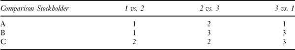
While the technical nature of Arrow's argument lies far beyond the scope of this book, an example can be used to illustrate something of the difficulties that arise in attempting to construct a firm's utility function. Table 20.3 tabulates the votes each project would receive if votes reflecting the preferences in Table 20.2 were made on a paired comparison basis. Such a basis is, at least to some persons, one reasonable way of attempting to resolve stockholder conflict. However, in the example given the approach fails. For in considering project 2 versus project 3, stockholders A and C would vote for project 2 and B for project 3. Other pairs are similarly ranked, as the table shows. But the table then indicates the presence of an intransitivity, because as a group the stockholders (when the votes are counted) prefer project 1 over project 2, 2 over 3, and 3 over 1. This means that as a group stockholders’ preferences are not consistent; the transitivity axiom (see Chapter 11) necessary for existence of a utility function is not satisfied. For this reason, a group utility function cannot exist in the present case, and management cannot resolve the conflicting preferences to the satisfaction of all stockholders. Arrow's work shows that all democratic schemes for resolving conflicts, such as the voting scheme just examined, can encounter this same difficulty.
TABLE 20.2 STOCKHOLDER RANKINGS OF MUTUALLY EXCLUSIVE PROJECTSa

aA ranking of 1 indicates the stockholder's most preferred project.
TABLE 20.3 STOCKHOLDER VOTING ON A PAIRED COMPARISON BASIS
20.4.2 When a Firm's Utility Function Does Exist
While a firm's utility function does not always exist, we can say that it will, if, loosely speaking, the stockholders are not too dissimilar in their preferences. On the one hand, this statement means that if stockholders use roughly similar rankings, conflicts can be resolved. The same is true if stockholders are exactly similar in either their attitudes toward risk or in their expectations regarding the future. We next examine each of these cases in turn. This provides some information about the conditions under which managers can be reasonably confident of acting in the shareholders’ best interests even if the market value criterion is not used.
20.4.2.1 Single-Peakedness Condition
To explain the notion of similarity between rankings, consider Figure 20.4, which plots each stockholder's ranking of the preferences indicated in Table 20.2 against the projects, which are arranged in numerical order. In the graph, we plot each stock-holder's rankings against the project numbers.13 We can see that project 2 is the least preferred of the three by stockholder B and the most preferred of the three by stockholder C. It can be shown by advanced methods, beyond the scope of this text, that in the present case our difficulty with paired comparison schemes resides in the attitudes of stockholder B. Moreover, it can be shown that if B's preferences are such that B's graph has a single high point (rather than a single low point as in Figure 20.4), then voting according to the paired comparison schemes will yield a transitive ranking that management can use in deriving a firm utility function. To see this by an example, suppose in Table 20.2 the rankings of stockholder B are replaced either by those of A or of C or by ranking the three projects in reverse order, that is, 3, 2, 1. If B uses any one of these three rankings, then paired voting will select a single project as most preferred by all three stockholders. If the ranking is 3, 2, 1, then in Table 20.3 stockholder B's votes would be recorded under 2 in the first comparison, under 3 in the second, and again under 3 in the third. This means the group now prefers 2 to 1, 2 to 3, and 1 to 3, so that project 2 can be selected by management.
FIGURE 20.4 STOCKHOLDER B'S PREFERENCES DO NOT EXHIBIT THE SINGLE-PEAKEDNESS PROPERTY

Accordingly, the example has suggested that if in a graph like Figure 20.4 no stockholder's ranking displays a low point in the middle of the set of projects ranked (technically if every stockholder's preferences are single-peaked), then a voting scheme to resolve conflicts of interest can be used. That is, the difficulties discovered by Arrow do not obtain when preferences are single-peaked. Hence, in such cases management can act in the best interests of all stockholders by following procedures along the lines indicated above. While such an approach might not be at all easy to put into practice, at least it does show that management will not always be paralyzed by inconsistent stockholder preferences. The importance of this possibility to practical decision making has been pointed out by Scott (1978).
Under more restrictive conditions than single peakedness, more can be said about a firm's utility function. A well-defined utility function for the firm exists either if (1) all stockholders’ preferences are identical, or if (2) their preferences are not identical but their expectations about the future are exactly the same.
20.4.2.2 Implications of Using a Firm's Utility Function
We have now identified three conditions that may justify substituting a firm utility function for the market value of its shares. These conditions are (1) that every stockholders’ preferences are single-peaked, or (2) that all stockholders’ preferences are identical, or (3) that if condition 2 does not hold, then stockholder expectations about the future must all be the same. Of course, if (2) does hold, a utility will also exist if stockholder expectations are identical. The point is that one of conditions (1), (2), or (3) must be satisfied for a utility to exist. Then, if both (2) and (3) are satisfied, the utility will certainly exist. Moreover, in the second and third instances we have indicated how the firm's utility is related to that of the individual stockholders.14
The foregoing conditions may obtain if either the past actions of the firm's management have attracted like-minded investors, or past policies have induced a particular set of expectations. To the extent that such conditions are satisfied, they tend to argue for gradual changes in financial policy so that dissatisfied investors can adjust their investment positions over time. It is probably most helpful if a firm's policy changes can be announced in advance, since given advance knowledge dissatisfied investors might be able to adjust their positions at lower transactions costs than would otherwise be the case.
20.4.3 Using Utilities When it is Possible
When a utility function for the firm does exist, management can use expected utility maximization as a decision criterion. That is, management can select actions that maximize the firm's expected utility rather than its market value. As we showed in the previous section, the manager considers the effects of actions on the distribution of cash flows, performs expected utility calculations for the distributions implied by available alternative actions (including different levels of investment), and selects an act that maximizes expected utility.
The use of expected utility maximization is more practical than it may first appear because such calculations can be approximated using risk-adjusted rates of return. To see this, consider the following example. Suppose the utility function is given by:
u(w)= w1/2
and consider a lottery, X, that pays $1 and $4 at time 2 with equal probability. Then:
![]()
A certainty equivalent c is defined by the condition:
![]()
Replacing the utility function by its explicit form, we obtain:
![]()
Squaring both sides of the above equation then gives:
![]()
But ![]() , so that the implied risk premium is
, so that the implied risk premium is ![]() The risk premium is measured at time 2, so that
The risk premium is measured at time 2, so that ![]() is a certainty equivalent value at time 2. Also suppose that the investment's certainty equivalent has a time 1 value15 of
is a certainty equivalent value at time 2. Also suppose that the investment's certainty equivalent has a time 1 value15 of ![]() , that is, the risk-free rate is 0.125 =
, that is, the risk-free rate is 0.125 = ![]() : Based on these assumptions, the risk-adjusted rate of return for the project is:
: Based on these assumptions, the risk-adjusted rate of return for the project is:

Accordingly, using expected utilities in one-period problems gives results similar to those obtained using risk-adjusted discount rates.16 The main problem with this approach is that unless the utility function's form is known, the firm's management does not know which risk-adjusted rate of return to choose. But if projects are acceptable over a range of risk-adjusted discount rates, management can be reasonably confident of their acceptability to the firm's stockholders. Note, moreover, that the lowest rate of discount the manager should use for risk-averse stockholders is certainly not less than the risk-free rate, that is, the rate that would be used by risk-neutral stockholders.
At this point one might ask whether there is really any difference between the present interpretation of expected utility maximization as implying risk-adjusted discount rates or the use of the CAPM to find the risk-adjusted rates according to which share prices are determined by discounting expected future earnings. From a policy point of view, there may not appear to be substantial differences between the two approaches—in both cases the size of the risk adjustment increases with the risk of the lottery being valued. Thus, the differences between the approaches are mainly conceptual, although the utility function approach does not require using any specific description of risk such as a covariance. Rather, the project distribution of return is used.
The real importance of our discussion of risk-adjusted rates thus becomes the implicit question of whose risk adjustment is to be used. If the CAPM is valid, market risk adjustments are to be used; if the expected utility model for a group of stockholders is valid, it is their risk adjustments that are of greatest importance to a firm's management. In either case, the tools we have developed indicate how to approach the problem of calculating the adjustments.
20.4.4 Using Dominance Criteria When Utilities are not Fully Specified
While in Section 20.4.3 it was suggested that the prescriptions of expected utility maximization could be approximated by risk-adjusted discount rates, there are also circumstances in which management can make decisions without knowing a great deal about stockholders’ utilities. Some, but not all, probability distributions can be compared for any utility function that, say, merely exhibits risk aversion.17 Thus, when management can only make weak assumptions about individual stockholders’ preferences (rather than postulate the exact nature of their utilities), decisions can sometimes still be made on behalf of them all in the knowledge that the stockholders would all approve. To see how this thinking applies to risk-averse stockholders, we consider first a simple situation applying whenever stockholders can be assumed to be materialistic in the sense of preferring more money to less. No assumptions about risk aversion will be required in this first example. However, after having considered this simple case, we shall then discuss a rule for use by management acting on behalf of risk-averse stockholders.
If management is willing only to assume that every stockholder's utility increases with wealth, there are still some lotteries that are clearly better than others irrespective of the utilities’ particular forms. For example, consider the following two lotteries, A and B, with payoffs and associated probabilities shown:
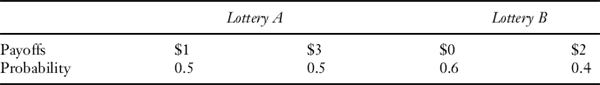
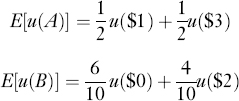
From Figure 20.5 it appears that lottery A would be preferred to lottery B, because lottery A always offers outcomes below a given fixed amount with lower probability than does lottery B (the downside risk of lottery A is lower).
To verify that this result is true for any decision maker whose utility increases with wealth, consider:
Then, under the assumption that utility increases in wealth,
![]()
FIGURE 20.5 FIRST-DEGREE STOCHASTIC DOMINANCE
E[u(A)] = E[u(B)]
As the example suggests, a choice between two lotteries can be made on the basis of these ideas whenever their respective distributions do not cross.18 Hence, if this were the only available ranking rule, in many cases it would mean that no comparisons could be made. However, sometimes this inability to compare distributions whose graphs cross can be resolved by imposing additional assumptions about stockholder preferences.
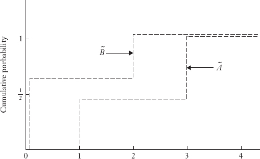
Hence, we now suppose all stockholders are risk averse in addition to preferring more wealth to less. Then we assume that management must compare lotteries C and D with the payoffs and probabilities shown below:
These are lotteries whose cumulative distributions cross as shown in Figure 20.6. As we showed in Chapter 9 (pages 187–188), in this case Lottery D is preferred by second degree stochastic dominance. For convenience the reasoning is repeated here. Notice first that E(D) = $![]() and E (C) = $2, so the risk-neutral stockholder at least would prefer lottery D. Note also that the worst outcome of lottery D is at least as good as (in fact better than) the worst outcome19 from lottery C. This means that in terms of the greatest possible downside risk, lottery D is never quite as bad as lottery C.
and E (C) = $2, so the risk-neutral stockholder at least would prefer lottery D. Note also that the worst outcome of lottery D is at least as good as (in fact better than) the worst outcome19 from lottery C. This means that in terms of the greatest possible downside risk, lottery D is never quite as bad as lottery C.
To see how it might be shown formally that lottery D is actually preferred by any risk-averter, let us ask if E[u(D)] = E[u(C)]. If it were, we would have:
![]()
which may also be written as:
![]()
Then after cancelling common terms and regrouping, we would have:
![]()
But u($1) − u($0) > u($2) − u($1) by the diminishing marginal utility characteristic of risk-averters, so the original inequality will certainly be satisfied if we can show that
![]()
But this expression reduces to
![]()
which is obviously true. Accordingly, it is now easy, by working backward from the last line, to verify that E[u(D)] < E[u(C)]; that is, lottery D is preferred to lottery C by all risk-averse decision makers.
The test for this relationship, known as second-degree stochastic dominance, which was described in Chapter 12, can be made systematically as follows. If, proceeding from the left in a graph like Figure 20.6, the area accumulated from the left of the graph and between the two distributions never changes sign,20 the distribution beginning on the right is said to be preferred according to the relationship of second-degree stochastic dominance.21 The method of making the calculations is displayed in the figure.
FIGURE 20.6 SECOND-DEGREE STOCHASTIC DOMINANCE (START EVALUATION AT LEFT-HAND SIDE OF THE DIAGRAM BECAUSE RISK-AVERSE INVESTORS ATTACH A GREATER NEGATIVE WEIGHT TO DOWNSIDE RISK THAN THEY DO TO UPSIDE POTENTIAL)

FIGURE 20.7 CHECKING FOR SECOND-DEGREE DOMINANCE

Not everything can be ranked by second-degree dominance, for there are pairs of distributions such that the area of the difference between the distributions does change sign as these areas are cumulated from the left. For example, consider Figure 20.7, drawn to indicate the distributions for the two lotteries that have the same payoffs as lotteries C and D but different probability distributions:

Note that ![]() , so that on the basis of the mean (but not on the basis of lowest outcomes) lottery C might prove to be a dominant lottery. But Figure 20.7 shows that the areas test is not satisfied, so that we cannot choose between lottery C and lottery D without knowing more about the decision maker's preferences. A risk-neutral decision maker would prefer lottery C, but lottery D has a better lowest outcome than lottery C, so that a highly risk-averse22 decision maker would prefer lottery D. Hence, neither lottery C nor lottery D satisfies the two conditions necessary for one to dominate the other.
, so that on the basis of the mean (but not on the basis of lowest outcomes) lottery C might prove to be a dominant lottery. But Figure 20.7 shows that the areas test is not satisfied, so that we cannot choose between lottery C and lottery D without knowing more about the decision maker's preferences. A risk-neutral decision maker would prefer lottery C, but lottery D has a better lowest outcome than lottery C, so that a highly risk-averse22 decision maker would prefer lottery D. Hence, neither lottery C nor lottery D satisfies the two conditions necessary for one to dominate the other.
FIGURE 20.8 PREFERENCE RELATIONS AND RANKING POSSIBILITIES

The findings may be summarized as follows. Management can rank some probability distributions by making only minimal assumptions about the preferences of stockholders on whose behalf the distributions are ranked. While not all distributions can be ranked by either of the criteria discussed here, more can be compared as the assumptions about stockholder preferences are made more specific. The relations between assumptions regarding preferences on the one hand and the classes of variables that can be ranked are displayed schematically in Figure 20.8. That is, the more things we are willing to specify about stockholders’ preferences, the larger the set of distributions we can compare. For example, if we assume stockholders are risk averse, we can use second-degree stochastic dominance23 to make at least some comparisons among prospects on behalf of the risk-averse stockholders.
20.5 MOTIVATING MANAGERS TO MEET OWNERS’ OBJECTIVES: AGENCY THEORY
If it is not easy to monitor the activities of managers, say because information about their performance is difficult to obtain, it becomes important to motivate managers to act in the best interests of the stockholders. Essentially, the problem is to ensure that management is motivated to maximize the criterion stockholders prefer. Incentive schemes can create this motivation by rewarding the manager for following stockholders’ preferences. For example, a stock option plan for management gives managers greater incentive to maximize share price than does a fixed salary arrangement that is independent of the firm's profit performance.
However, such schemes resolve the motivation problem only partially. One reason for a potential conflict between stockholders’ and managers’ objectives, even with stock options24 or other forms of profit sharing, is that a manager's compensation may be tied entirely to the fortunes of the firm. Recall that we earlier divided the firm's standard deviation of return into diversifiable and nondiversifiable components. Since stockholders normally purchase a firm's shares as part of a portfolio, only a stock's systematic risk is of concern to them, at least in markets that are perfect or nearly so. But if managers are less able to diversify their personal investments,25 they may be concerned with unsystematic risk as well. This could lead them to make operating (investment) decisions that are less risky than would be optimal from the stockholders’ viewpoints.26
This problem has been studied using the economic theory of agency.27 The stockholders’ (principal's) problem is to design a compensation scheme that will lead an expected utility-maximizing manager (agent) to maximize the principal's expected utility. The current state of the approach is rather abstract and thus beyond the scope of this text. Nevertheless, it does suggest that the owners’ problem of contracting for the services of a manager may fruitfully be examined as a problem in buying information. In this case the information purchased is the manager's opinion regarding possible excess returns from the operation, and its price is the manager's fee. The fee to be paid will depend on whether the owner can evaluate the excess returns correctly. If so, the fee will be less than otherwise (the owner and manager engage in the form of bargaining known as bilateral monopoly, so the outcome is indeterminate a priori). The analysis by Heckerman (1975) shows that if the manager is allowed to invest in the firm (stock option), he will value the option less as the standard deviation of the firm's return increases, requiring a larger fixed fee in compensation. The owner's protection lies in keeping the fixed fee small enough so that the manager will accept the contract only if the manager believes the excess return is large enough to protect the owner. Such a participatory contract between an owner and a manager will require a higher rate of return for investment decisions than otherwise to compensate the owner for the costs of obtaining the information needed to design the contract.
Another approach emphasizing the costs of monitoring agency relationships has been developed by Jensen and Meckling (1976). These authors argue that managers of firms can always take some of their income in kind, since the cost to the stockholders of monitoring an agent's every action would be prohibitively great. The problem, then, becomes one of balancing off incentives paid to agents against the costs of monitoring those actions for which incentives to act in the stockholders’ best interests are not provided.
KEY POINTS
- Capital market imperfections have far-reaching implications for financial decision making.
- There are several kinds of capital market imperfections: heterogeneous expectations, unequally distributed information, transactions costs, tax differentials, and the costs of unsystematic risk.
- With heterogeneous expectations, investors have differences of opinion regarding the probability distributions of future events.
- Assuming heterogeneous expectations weakens but does not destroy the CAPM notion of a risk-return trade-off. However, the risk-return trade-offs faced by a given investor may not correspond to those of the capital market line.
- In addition to heterogeneous expectations regarding the future, investors may not even share the same information about the past. Therefore, it may be difficult for potential investors to accurately evaluate the nature of the risks involved in purchasing the securities of some firms. Similarly, in debt markets it may be difficult for lenders to assess accurately the credit risk of borrowers.
- The major imperfection affecting market prices appears to involve the collection and dissemination of information that seems often to be distributed quite unevenly.
- When capital markets are not perfect, the market value of the firm is not always well defined and therefore management action to maximize stockholder value is not always as clear as in the case of a perfect capital market.
- In an imperfect capital market, financial and operating decisions are no longer separable, because the value of the firm depends on both the operating decision, which determines the amount of financing needed, and the manner in which the funds are raised. Therefore, the effects of investment and financing decisions must be assessed in combination.
- In a world of capital market imperfections, a firm's market value is not uniquely determined by a fixed relationship between risk and return, because management has no ready way of using market rates of return to judge the effect of its actions on the well-being of the firm's stockholders.
- In an imperfect capital market, firm investing decisions are more difficult for management because the firm does not necessarily have a unique cost of capital that it can use as a hurdle rate in deciding on the acceptability of investment projects.
- While the usefulness of the market value rule in a perfect capital market is its ability to provide a standard reflecting the best interests of all the firm's stockholders, this standard is impaired because of capital market imperfections.
- In an imperfect capital market, the difficulty faced by management is in knowing what to do if a firm's owners have conflicting preferences, because under reasonable conditions regarding preferences no rule for resolving conflicts may exist.
- When operating in an imperfect capital market, a firm's management must maximize a criterion function by choosing operating and financial decisions in combination.
- Two ways for management to deal with unevenly distributed information are via signals and through contingency planning.
- A firm's utility function representing the best interests of all stockholders need not always exist. The conflicting preferences of individual stockholders are not always capable of being resolved, at least in any democratic fashion. In fact, it has been shown that it is not generally possible to resolve conflicting preferences without acting in an essentially dictatorial fashion.
- There are conditions that may justify substituting a firm's utility function for the market value of its shares. If a firm's utility function can be employed, management can use expected utility maximization as a decision criterion.
- The expected utility maximization approach that management can follow in an imperfect capital market could be approximated by using a risk-adjusted discount rate. Moreover, there are circumstances in which management can make decisions without knowing a great deal about stockholders’ utilities.
- Incentive schemes (such as stock option plans) must be designed to motivate managers for following the preferences of stockholders. The stockholders’ (principal's) problem is to design a compensation scheme that will lead an expected utility-maximizing manager (agent) to maximize the principal's expected utility.
QUESTIONS
- What are some circumstances in which differences in expectations might result in stock prices being lower than in the case of investor agreement?
- What are the implications of unequally distributed information for investors and the management of a firm?
- Because of a concern with unsystematic risk, a firm's management might be tempted to operate the firm in a manner not wholly consistent with stockholder interests. Can you think of a financial arrangement that might partly alleviate this problem?
- If mutual funds can effect diversification more cheaply than individual investors, they might be able to earn greater returns on a portfolio of given risk than would individual investors. Assuming this to be true, who would be likely to receive the excess returns, and why? (Hint: Specify carefully the market conditions in which the mutual funds are assumed to trade.)
- Why is there a need for an integrated approach to financial decision making?
- What are the conditions that may justify substituting the market value of a company's shares for its utility function?
- In an imperfect capital market, can the managers of a firm still use the market value of the company as a rule for making decisions? If not, what other criterion can they use to make financial decisions?
- The management of Minuscule Investments Ltd. is considering two investment proposals, X and Y, either of which may be had for $10 million. Because of a limited capital budget, only one of the two can be selected. Their one-period payoffs are, respectively,
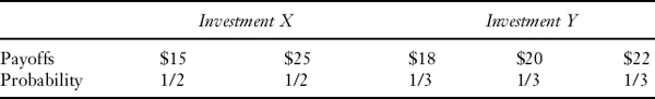
Which set of payoffs is preferable and why? (Hint: Consider second-degree stochastic dominance in answering this question.)
- You are asked to compare the following probability distributions of cash flows:
- A versus B:
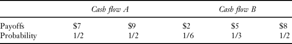
- C versus D:

- E versus F:
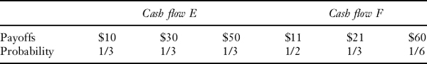
What comparisons can you make in each case, and why?
- A versus B:
- The stockholders’ utility function for a firm is
 . Assuming that the risk-free rate is 10%, determine the risk-adjusted return of a lottery that pays $2 with probability
  and $6 with probability
  .
. - Let's suppose that the risk adjustment of investors is 0.05% and the risk-free rate is 4%. Determine the time 1 value of the following contingent claim in the different cases:

- Homogenous expectations and risk-neutral investor
- Homogenous expectations and risk-averse investor
- Now suppose a market with two identical claims and three investors and let's assume that an investor can hold at most one claim. Let's also suppose that the investors have the following view of the contingent claim:

What will be the price of the contingent claim in this market?
REFERENCES
Akerlof, George A. (1976). “The Economics of Caste and of the Rat Race and Other Woeful Tales,” Quarterly Journal of Economics 90: 599–617.
Arrow, Kenneth J. (1951). Social Choice and Individual Value. New York: John Wiley & Sons.
Friend, Irwin, and James R. Bicksler. (1977). Risk and Return in Finance. Cambridge, MA: Ballinger.
Hadar, Josef, and William R. Russell. (1969). “Rules for Ordering Uncertain Prospects,” American Economic Review 59: 24–35.
Heckerman, Donald G. (1975). “Motivating Managers to Make Investment Decisions,” Journal of Financial Economics 2: 273–292.
Jaffee, Dwight M., and Thomas Russell. (1976). “Imperfect Information, Uncertainty, and Credit Rationing,” Quarterly Journal of Economics 90: 651–666.
Jensen, Michael C., and William M. Meckling. (1976). “Theory of the Firm: Managerial Behavior, Agency Costs, and Ownership Structure,” Journal of Financial Economics 3: 305–360.
Lintner, John. (1969). “The Aggregation of Investors’ Diverse Judgments and Preferences in Purely Competitive Security Markets,” Journal of Financial and Quantitative Analysis 4: 347–400.
Miller, Edward M. (1977). “Risk, Uncertainty, and Divergence of Opinion,” Journal of Finance 32: 1151–1167.
Miller, Edward M. (2004a). “Restrictions on Short Selling and Exploitable Opportunities for Investors,” in Frank J. Fabozzi (ed.), Short Selling: Strategies, Risks, and Rewards. Hoboken, NJ: John Wiley & Sons.
Miller, Edward M. (2004b). “Implications of Short Selling and Divergence of Opinion for Investment Strategy,” in Frank J. Fabozzi (ed.), Short Selling: Strategies, Risks, and Rewards. Hoboken, NJ: John Wiley & Sons.
Miller, Edward M. (2004c). “Short Selling and Financial Puzzle,” in Frank J. Fabozzi (ed.), Short Selling: Strategies, Risks, and Rewards. Hoboken, NJ: John Wiley & Sons.
Salop, Joanne and Steven Salop. (1976). “Self-Selection and Turnover in the Labor Market,” Quarterly Journal of Economics 90: 619–627.
Scott, William R. (1978). “Group Preference Orderings for Audit and Valuation Alternatives: The Single-Peakedness Condition,” Accounting Review 53: 120–137.
Williamson, Oliver E. (1975). Markets and Hierarchies: Economic Analysis and Antitrust Implications. New York: Free Press.
Wilson, Robert. (1968). “The Theory of Syndicates,” Econometrica 36: 119–132.
1 This will normally be the case in a two-state world if state 1 is associated with favorable economic conditions.
2 The thinking underlying this example is due to Edward Miller (1977). Compare Miller's Figure 1.
3 Miller (1977, p. 1153). We cite only some of the conclusions reached in the original article. For extension of this work, see Miller (2004a, 2004b, 2004c).
4 This means an increase in dispersion of opinions while the mean of the distribution remains constant.
5 These situations are examples of a condition termed information impactedness, and the insurance scenario also illustrates a situation known as moral hazard that we mentioned in Chapter 1 and discuss further in the next chapter. For further discussion of these important concepts, see Williamson (1975).
6 See Jaffee and Russell (1976).
7 This point takes on special importance when it is recognized that employers (boards of directors) may not always know exactly the capacities of their employees (the firm's management). For discussions of difficulties with such agency relations, see Akerlof (1976) and Salop (1976).
8 See Lintner (1969). The market price of risk becomes, in effect, a weighted average of individual investors’ risk-return trade-offs. The security market line is explained in Chapter 14.
9 Miller (1977, p. 1157) summarizes evidence suggesting that the riskiest stocks in the market will tend to plot below the capital market line. For further discussion, see Friend and Bicksler (1977).
10 These results will be established in Section 20.4.
11 This argument is due to Williamson (1975). On the other hand, Miller (1977, p. 1162) suggests that with heterogeneous expectations, the total market value of two otherwise independent firms can be lowered by a conglomerate merger.
12 If the amounts of funds involved are large, alternative organizations such as investment clubs with many members might not be able to perform the same task. Moreover, an investment club will not usually have the same supervisory capabilities as a conglomerate headquarters staff. Williamson (1975) attaches considerable weight to conglomerates’ supervisory capabilities.
13 The height of a particular stockholder's preferences is not relevant. The essential feature of the graph is how a given stockholder ranks the projects relative to each other, that is, the slope of the individual stockholder's graph showing preferences.
14 For a full discussion, see Wilson (1968).
15 That is, if the risk-free rate is 0.125 = 1/8.
16 Caution: The use of risk-adjusted rates in multiperiod models can lead to incorrect decisions unless carefully interpreted. We discuss these issues in Chapter 25.
17 See also the discussion of stochastic dominance in Chapter 12.
18 The relationship between lottery A and lottery B is in this case expressed by saying lottery A dominates lottery B in the first degree. See Hadar and Russell (1969) for a proof of the general result.
19 These are necessary conditions for the ranking we are now establishing, second-degree dominance. They are necessary to prevent lottery D from being rejected by risk-averters who are especially heavily influenced by worst-case thinking. Note that these necessary conditions do not imply σ2(D) must always be smaller than σ2(C).
20 Individual components of the accumulated area may differ in sign, as Figure 20.7 shows. It is only the accumulated area that must always have the same sign.
21 Formal proofs of this result are given in Hadar and Russell (1969).
22 Technically this holds if the decision maker's index of absolute risk aversion is sufficiently large.
23 For further discussion of the dominance concepts, see Chapter 12.
24 Companies are rethinking the use of stock options, in part because of backdated options scandals. A backdated option is an executive option grant in which the date of the grant has been manipulated to provide greater benefits to the executive and to minimize taxes. Such manipulation, however, violates financial disclosure and tax laws.
25 This is because through a stock option plan their major investment may be in the firm they manage.
26 In terms of the transformation curve of Chapter 2, it is not shifted up and to the right as far as it could be. Recall we stated that it was the manager's technical knowledge of the firm's operations that established the position of this curve.
27 See Heckerman (1975).