
CHAPTER 20
Numeric Linear Algebra

This chapter deals with two main topics. The first topic is how to solve linear systems of equations numerically. We start with Gauss elimination, which may be familiar to some readers, but this time in an algorithmic setting with partial pivoting. Variants of this method (Doolittle, Crout, Cholesky, Gauss–Jordan) are discussed in Sec. 20.2. All these methods are direct methods, that is, methods of numerics where we know in advance how many steps they will take until they arrive at a solution. However, small pivots and roundoff error magnification may produce nonsensical results, such as in the Gauss method. A shift occurs in Sec. 20.3, where we discuss numeric iteration methods or indirect methods to address our first topic. Here we cannot be totally sure how many steps will be needed to arrive at a good answer. Several factors—such as how far is the starting value from our initial solution, how is the problem structure influencing speed of convergence, how accurate would we like our result to be—determine the outcome of these methods. Moreover, our computation cycle may not converge. Gauss–Seidel iteration and Jacobi iteration are discussed in Sec. 20.3. Section 20.4 is at the heart of addressing the pitfalls of numeric linear algebra. It is concerned with problems that are ill-conditioned. We learn to estimate how “bad” such a problem is by calculating the condition number of its matrix.
The second topic (Secs. 20.6–20.9) is how to solve eigenvalue problems numerically. Eigenvalue problems appear throughout engineering, physics, mathematics, economics, and many areas. For large or very large matrices, determining the eigenvalues is difficult as it involves finding the roots of the characteristic equations, which are high-degree polynomials. As such, there are different approaches to tackling this problem. Some methods, such as Gerschgorin's method and Collatz's method only provide a range in which eigenvalues lie and thus are known as inclusion methods. Others such as tridiagonalization and QR-factorization actually find all the eigenvalues. The area is quite ingeneous and should be fascinating to the reader.
Prerequisite: Secs. 7.1, 7.2, 8.1.
Sections that may be omitted in a shorter course: 20.4, 20.5, 20.9.
References and Answers to Problems: App. 1 Part E, App. 2.
20.1 Linear Systems: Gauss Elimination
The basic method for solving systems of linear equations by Gauss elimination and back substitution was explained in Sec. 7.3. If you covered Sec. 7.3, you may wonder why we cover Gauss elimination again. The reason is that here we cover Gauss elimination in the setting of numerics and introduce new material such as pivoting, row scaling, and operation count. Furthermore, we give an algorithmic representation of Gauss elimination in Table 20.1 that can be readily converted into software. We also show when Gauss elimination runs into difficulties with small pivots and what to do about it. The reader should pay close attention to the material as variants of Gauss elimination are covered in Sec. 20.2 and, furthermore, the general problem of solving linear systems is the focus of the first half of this chapter.
A linear system of n equations in n unknowns x1, …, xn is a set of equations E1, …, En of the form
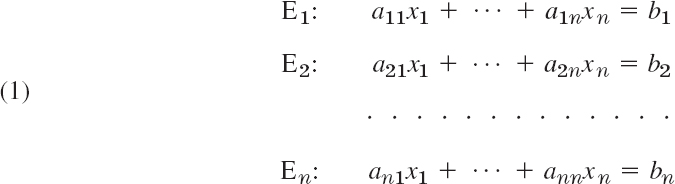
where the coefficients ajk and the bj are given numbers. The system is called homogeneous if all the bj are zero; otherwise it is called nonhomogeneous. Using matrix multiplication (Sec. 7.2), we can write (1) as a single vector equation
![]()
where the coefficient matrix A = [ajk] is the n × n matrix
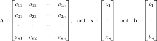
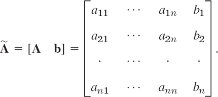
are column vectors. The following matrix ![]() is called the augmented matrix of the system (1):
is called the augmented matrix of the system (1):
A solution of (1) is a set of numbers x1, …, xn that satisfy all the n equations, and a solution vector of (1) is a vector x whose components constitute a solution of (1).
The method of solving such a system by determinants (Cramer's rule in Sec. 7.7) is not practical, even with efficient methods for evaluating the determinants.
A practical method for the solution of a linear system is the so-called Gauss elimination, which we shall now discuss (proceeding independently of Sec. 7.3).
Gauss Elimination
This standard method for solving linear systems (1) is a systematic process of elimination that reduces (1) to triangular form because the system can then be easily solved by back substitution. For instance, a triangular system is
and back substitution gives ![]() from the third equation, then
from the third equation, then
![]()
from the second equation, and finally from the first equation
![]()
How do we reduce a given system (1) to triangular form? In the first step we eliminate x1 from equations E2 to En in (1). We do this by adding (or subtracting) suitable multiples of E1 to (from) equations E2, …, En and taking the resulting equations, call them ![]() as the new equations. The first equation, E1, is called the pivot equation in this step, and a11 is called the pivot. This equation is left unaltered. In the second step we take the new second equation
as the new equations. The first equation, E1, is called the pivot equation in this step, and a11 is called the pivot. This equation is left unaltered. In the second step we take the new second equation ![]() (which no longer contains x1) as the pivot equation and use it to eliminate x2 from
(which no longer contains x1) as the pivot equation and use it to eliminate x2 from ![]() to
to ![]() . And so on. After n − 1 steps this gives a triangular system that can be solved by back substitution as just shown. In this way we obtain precisely all solutions of the given system (as proved in Sec. 7.3).
. And so on. After n − 1 steps this gives a triangular system that can be solved by back substitution as just shown. In this way we obtain precisely all solutions of the given system (as proved in Sec. 7.3).
The pivot akk (in step k) must be different from zero and should be large in absolute value to avoid roundoff magnification by the multiplication in the elimination. For this we choose as our pivot equation one that has the absolutely largest ajk in column k on or below the main diagonal (actually, the uppermost if there are several such equations). This popular method is called partial pivoting. It is used in CASs (e.g., in Maple).
Partial pivoting distinguishes it from total pivoting, which involves both row and column interchanges but is hardly used in practice.
Let us illustrate this method with a simple example.
EXAMPLE 1 Gauss Elimination. Partial Pivoting
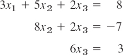
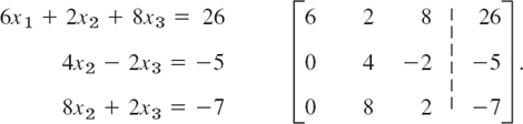
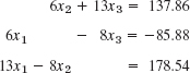
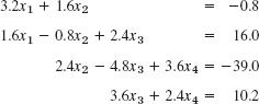
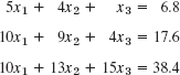
Solve the system

Solution. We must pivot since E1 has no x1-term. In Column 1, equation E3 has the largest coefficient. Hence we interchange E1 and E3,

It would suffice to show the augmented matrix and operate on it. We show both the equations and the augmented matrix. In the first step, the first equation is the pivot equation. Thus

To eliminate x1 from the other equations (here, from the second equation), do:
![]()
The result is
Step 2. Elimination of x2
The largest coefficient in Column 2 is 8. Hence we take the new third equation as the pivot equation, interchanging equations 2 and 3,
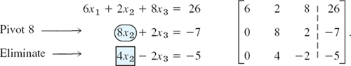
To eliminate x2 from the third equation, do:
![]()
The resulting triangular system is shown below. This is the end of the forward elimination. Now comes the back substitution.
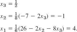
Back substitution. Determination of x3, x2, x1
The triangular system obtained in Step 2 is

From this system, taking the last equation, then the second equation, and finally the first equation, we compute the solution
This agrees with the values given above, before the beginning of the example.
The general algorithm for the Gauss elimination is shown in Table 20.1. To help explain the algorithm, we have numbered some of its lines. bj is denoted by aj,n+1, for uniformity. In lines 1 and 2 we look for a possible pivot. [For k = 1 we can always find one; otherwise x1 would not occur in (1).] In line 2 we do pivoting if necessary, picking an ajk of greatest absolute value (the one with the smallest j if there are several) and interchange the corresponding rows. If |akk| is greatest, we do no pivoting. mjk in line 4 suggests multiplier, since these are the factors by which we have to multiply the pivot equation ![]() in Step k before subtracting it from an equation
in Step k before subtracting it from an equation ![]() below
below ![]() from which we want to eliminate xk. Here we have written
from which we want to eliminate xk. Here we have written ![]() and
and ![]() to indicate that after Step 1 these are no longer the equations given in (1), but these underwent a change in each step, as indicated in line 5. Accordingly, ajk etc. in all lines refer to the most recent equations, and j
to indicate that after Step 1 these are no longer the equations given in (1), but these underwent a change in each step, as indicated in line 5. Accordingly, ajk etc. in all lines refer to the most recent equations, and j ![]() k in line 1 indicates that we leave untouched all the equations that have served as pivot equations in previous steps. For p = k in line 5 we get 0 on the right, as it should be in the elimination,
k in line 1 indicates that we leave untouched all the equations that have served as pivot equations in previous steps. For p = k in line 5 we get 0 on the right, as it should be in the elimination,

In line 3, if the last equation in the triangular system is ![]() we have no solution. If it is
we have no solution. If it is ![]() we have no unique solution because we then have fewer equations than unknowns.
we have no unique solution because we then have fewer equations than unknowns.
EXAMPLE 2 Gauss Elimination in Table 20.1, Sample Computation
In Example 1 we had a11 = 0, so that pivoting was necessary. The greatest coefficient in Column 1 was a31. Thus ![]() in line 2, and we interchanged E1 and E3. Then in lines 4 and 5 we computed
in line 2, and we interchanged E1 and E3. Then in lines 4 and 5 we computed ![]() and
and
![]()
and then ![]() , so that the third equation 8x2 + 2x3 = −7 did not change in Step 1. In Step 2 (k = 2) we had 8 as the greatest coefficient in Column 2, hence
, so that the third equation 8x2 + 2x3 = −7 did not change in Step 1. In Step 2 (k = 2) we had 8 as the greatest coefficient in Column 2, hence ![]() . We interchanged equations 2 and 3, computed
. We interchanged equations 2 and 3, computed ![]() in line 5, and the
in line 5, and the ![]() This produced the triangular form used in the back substitution.
This produced the triangular form used in the back substitution.
If akk = 0 in Step k, we must pivot. If |akk| is small, we should pivot because of roundoff error magnification that may seriously affect accuracy or even produce nonsensical results.
EXAMPLE 3 Difficulty with Small Pivots
The solution of the system

is x1 = 10, x2 = 1. We solve this system by the Gauss elimination, using four-digit floating-point arithmetic. (4D is for simplicity. Make an 8D-arithmetic example that shows the same.)
(a) Picking the first of the given equations as the pivot equation, we have to multiply this equation by m = 0.4003/0.0004 = 1001 and subtract the result from the second equation, obtaining
![]()
Hence x2 = −1404/(−1405) = 0.9993, and from the first equation, instead of x1 = 10, we get
![]()
This failure occurs because |a11| is small compared with |a12|, so that a small roundoff error in x2 leads to a large error in x1.
(b) Picking the second of the given equations as the pivot equation, we have to multiply this equation by 0.0004/0.4003 = 0.0009993 and subtract the result from the first equation, obtaining
![]()
Hence x2 = 1, and from the pivot equation x1 = 10. This success occurs because |a21| is not very small compared to |a22|, so that a small roundoff error in x2 would not lead to a large error in x1. Indeed, for instance, if we had the value x2 = 1.002, we would still have from the pivot equation the good value x1 = (2.501 + 1.505)/0.4003 = 10.01.

Error estimates for the Gauss elimination are discussed in Ref. [E5] listed in App. 1.
Row scaling means the multiplication of each Row j by a suitable scaling factor sj. It is done in connection with partial pivoting to get more accurate solutions. Despite much research (see Refs. [E9], [E24] in App. 1) and the proposition of several principles, scaling is still not well understood. As a possibility, one can scale for pivot choice only (not in the calculation, to avoid additional roundoff) and take as first pivot the entry aj1 for which |aj1|/|Aj| is largest; here Aj is an entry of largest absolute value in Row j. Similarly in the further steps of the Gauss elimination.
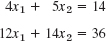
For instance, for the system

we might pick 4 as pivot, but dividing the first equation by 104 gives the system in Example 3, for which the second equation is a better pivot equation.
Operation Count
Quite generally, important factors in judging the quality of a numeric method are
Amount of storage
Amount of time (≡ number of operations)
Effect of roundoff error
For the Gauss elimination, the operation count for a full matrix (a matrix with relatively many nonzero entries) is as follows. In Step k we eliminate xk from n − k equations. This needs n − k divisions in computing the mjk (line 3) and (n − k)(n − k + 1) multiplications and as many subtractions (both in line 4). Since we do n − 1 steps, k goes from 1 to n − 1 and thus the total number of operations in this forward elimination is

where 2n3/3 is obtained by dropping lower powers of n. We see that f(n) grows about proportional to n3. We say that f(n) is of order n3 and write
![]()
where O suggests order. The general definition of O is as follows. We write
![]()
if the quotients |f(n)/h(n)| and |h(n)/f(n)| remain bounded (do not trail off to infinity) as n → ∞. In our present case, h(n) = n3 and, indeed, ![]() because the omitted terms divided by n3 go to zero as n → ∞.
because the omitted terms divided by n3 go to zero as n → ∞.
In the back substitution of xi we make n − i multiplications and as many subtractions, as well as 1 division. Hence the number of operations in the back substitution is

We see that it grows more slowly than the number of operations in the forward elimination of the Gauss algorithm, so that it is negligible for large systems because it is smaller by a factor n, approximately. For instance, if an operation takes 10−9 sec, then the times needed are:

APPLICATIONS of linear systems see Secs. 7.1 and 8.2.
1–3 GEOMETRIC INTERPRETATION
Solve graphically and explain geometrically.
4–16 GAUSS ELIMINATION
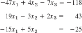
Solve the following linear systems by Gauss elimination, with partial pivoting if necessary (but without scaling). Show the intermediate steps. Check the result by substitution. If no solution or more than one solution exists, give a reason.
- 4.

- 5.

- 6.

- 7.
- 8.

- 9.
- 10.
- 11.

- 12.
- 13.

- 14.
- 15.

- 16.
- 17. CAS EXPERIMENT. Gauss Elimination. Write a program for the Gauss elimination with pivoting. Apply it to Probs. 13–16. Experiment with systems whose coefficient determinant is small in absolute value. Also investigate the performance of your program for larger systems of your choice, including sparse systems.
- 18. TEAM PROJECT. Linear Systems and Gauss Elimination. (a) Existence and uniqueness. Find a and b such that ax1 + x2 = b, x1 + x2 = 3 has (i) a unique solution, (ii) infinitely many solutions, (iii) no solutions.
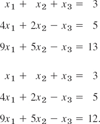
- (b) Gauss elimination and nonexistence. Apply the Gauss elimination to the following two systems and compare the calculations step by step. Explain why the elimination fails if no solution exists.
- (c) Zero determinant. Why may a computer program give you the result that a homogeneous linear system has only the trivial solution although you know its coefficient determinant to be zero?
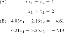
- (d) Pivoting. Solve System (A) (below) by the Gauss elimination first without pivoting. Show that for any fixed machine word length and sufficiently small
 > 0 the computer gives x2 = 1 and then x1 = 0. What is the exact solution? Its limit as → 0? Then solve the system by the Gauss elimination with pivoting. Compare and comment.
 - (e) Pivoting. Solve System (B) by the Gauss elimination and three-digit rounding arithmetic, choosing (i) the first equation, (ii) the second equation as pivot equation. (Remember to round to 3S after each operation before doing the next, just as would be done on a computer!) Then use four-digit rounding arithmetic in those two calculations. Compare and comment.
- (b) Gauss elimination and nonexistence. Apply the Gauss elimination to the following two systems and compare the calculations step by step. Explain why the elimination fails if no solution exists.
20.2 Linear Systems: LU-Factorization, Matrix Inversion
We continue our discussion of numeric methods for solving linear systems of n equations in n unknowns x1, …, xn,
![]()
where A = [ajk] is the n × n given coefficient matrix and xT = [x1, …, xn] and bT = [b1, …, bn]. We present three related methods that are modifications of the Gauss elimination, which require fewer arithmetic operations. They are named after Doolittle, Crout, and Cholesky and use the idea of the LU-factorization of A, which we explain first.
An LU-factorization of a given square matrix A is of the form

where L is lower triangular and U is upper triangular. For example,

It can be proved that for any nonsingular matrix (see Sec. 7.8) the rows can be reordered so that the resulting matrix A has an LU-factorization (2) in which L turns out to be the matrix of the multipliers mjk of the Gauss elimination, with main diagonal 1, …, 1, and U is the matrix of the triangular system at the end of the Gauss elimination. (See Ref. [E5], pp. 155–156, listed in App. 1.)
The crucial idea now is that L and U in (2) can be computed directly, without solving simultaneous equations (thus, without using the Gauss elimination). As a count shows, this needs about n3/3 operations, about half as many as the Gauss elimination, which needs about 2n3/3 (see Sec. 20.1). And once we have (2), we can use it for solving Ax = b in two steps, involving only about n2 operations, simply by noting that Ax = LUx = b may be written

and solving first (3a) for y and then (3b) for x. Here we can require that L have main diagonal 1, …, 1 as stated before; then this is called Doolittle's method.1 Both systems (3a) and (3b) are triangular, so we can solve them as in the back substitution for the Gauss elimination.
A similar method, Crout's method,2 is obtained from (2) if U (instead of L) is required to have main diagonal 1, …, 1. In either case the factorization (2) is unique.
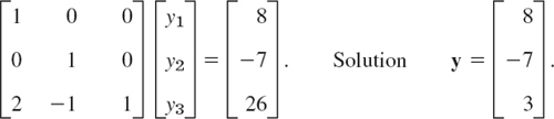
Solve the system in Example 1 of Sec. 20.1 by Doolittle's method.
Solution. The decomposition (2) is obtained from
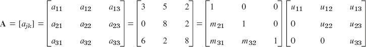
by determining the mjk and ujk, using matrix multiplication. By going through A row by row we get successively

Thus the factorization (2) is
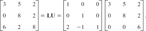
We first solve LY = b, determining y1 = 8, then y2 = −7, then y3 from 2y1 − y2 + y3 = 16 + 7 + y3 = 26; thus (note the interchange in b because of the interchange in A!)
Then we solve Ux = y, determining ![]() then x2, then x1, that is,
then x2, then x1, that is,

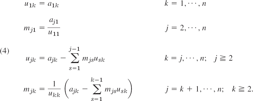
Our formulas in Example 1 suggest that for general n the entries of the matrices L = [mjk] (with main diagonal 1, …, 1 and mjk suggesting “multiplier”) and U = [ujk] in the Doolittle method are computed from
Row Interchanges. Matrices, such as

have no LU-factorization (try!). This indicates that for obtaining an LU-factorization, row interchanges of A (and corresponding interchanges in b) may be necessary.
Cholesky's Method
For a symmetric, positive definite matrix A (thus A = AT, xTAx > 0 for all x ≠ 0) we can in (2) even choose U = LT, thus ujk = mkj (but cannot impose conditions on the main diagonal entries). For example,
The popular method of solving Ax = b based on this factorization A = LLT is called Cholesky's method.3 In terms of the entries of L = [ljk] the formulas for the factorization are
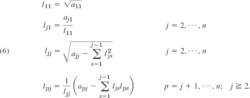
If A is symmetric but not positive definite, this method could still be applied, but then leads to a complex matrix L, so that the method becomes impractical.
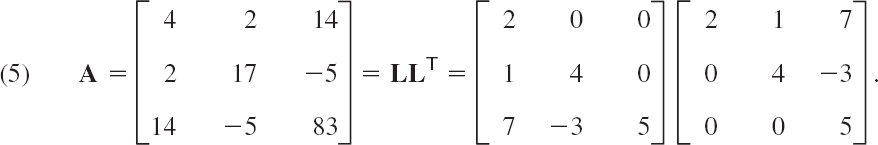
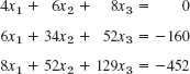
Solve by Cholesky's method:

Solution. From (6) or from the form of the factorization
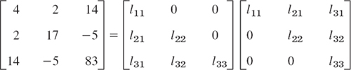
we compute, in the given order,

This agrees with (5). We now have to solve Ly = b, that is,
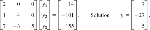
As the second step, we have to solve Ux = LTx = y, that is,

THEOREM 1 Stability of the Cholesky Factorization
The Cholesky LLT-factorization is numerically stable (as defined in Sec. 19.1).
PROOF
We have ![]() by squaring the third formula in (6) and solving it for ajj. Hence for all ljk (note that ljk = 0 for k > j) we obtain (the inequality being trivial)
by squaring the third formula in (6) and solving it for ajj. Hence for all ljk (note that ljk = 0 for k > j) we obtain (the inequality being trivial)
![]()
That is, ![]() is bounded by an entry of A, which means stability against rounding.
is bounded by an entry of A, which means stability against rounding.
Gauss–Jordan Elimination. Matrix Inversion
Another variant of the Gauss elimination is the Gauss–Jordan elimination, introduced by W. Jordan in 1920, in which back substitution is avoided by additional computations that reduce the matrix to diagonal form, instead of the triangular form in the Gauss elimination. But this reduction from the Gauss triangular to the diagonal form requires more operations than back substitution does, so that the method is disadvantageous for solving systems Ax = b. But it may be used for matrix inversion, where the situation is as follows.
The inverse of a nonsingular square matrix A may be determined in principle by solving the n systems
![]()
where bj is the jth column of the n × n unit matrix.
However, it is preferable to produce A−1 by operating on the unit matrix I in the same way as the Gauss–Jordan algorithm, reducing A to I. A typical illustrative example of this method is given in Sec. 7.8.
1–5 DOOLITTLE'S METHOD
Show the factorization and solve by Doolittle's method.


- TEAM PROJECT. Crout's method factorizes A = LU, where L is lower triangular and U is upper triangular with diagonal entries ujj = 1, j = 1, …, n.
(a) Formulas. Obtain formulas for Crout's method similar to (4).
(b) Examples. Solve Prob. 5 by Crout's method.
(c) Factor the following matrix by the Doolittle, Crout, and Cholesky methods.

(d) Give the formulas for factoring a tridiagonal matrix by Crout's method.
(e) When can you obtain Crout's factorization from Doolittle's by transposition?
7–12 CHOLESKY'S METHOD
Show the factorization and solve.
- 7.

- 8.
- 9.

- 10.
- 11.

- 12.

- 13. Definiteness. Let A, B be n × n and positive definite. Are −A, A, A + B, A − B positive definite?
- 14. CAS PROJECT. Cholesky's Method. (a) Write a program for solving linear systems by Cholesky's method and apply it to Example 2 in the text, to Probs. 7–9, and to systems of your choice.
- (b) Splines. Apply the factorization part of the program to the following matrices (as they occur in (9), Sec. 19.4 (with cj = 1), in connection with splines).

- (b) Splines. Apply the factorization part of the program to the following matrices (as they occur in (9), Sec. 19.4 (with cj = 1), in connection with splines).
15–19 INVERSE
Find the inverse by the Gauss–Jordan method, showing the details.
- 15. In Prob. 1
- 16. In Prob. 4
- 17. In Team Project 6(c)
- 18. In Prob. 9
- 19. In Prob. 12
- 20. Rounding. For the following matrix A find det A. What happens if you roundoff the given entries to (a) 5S, (b) 4S, (c) 3S, (d) 2S, (e) lS? What is the practical implication of your work?
20.3 Linear Systems: Solution by Iteration
The Gauss elimination and its variants in the last two sections belong to the direct methods for solving linear systems of equations; these are methods that give solutions after an amount of computation that can be specified in advance. In contrast, in an indirect or iterative method we start from an approximation to the true solution and, if successful, obtain better and better approximations from a computational cycle repeated as often as may be necessary for achieving a required accuracy, so that the amount of arithmetic depends upon the accuracy required and varies from case to case.
We apply iterative methods if the convergence is rapid (if matrices have large main diagonal entries, as we shall see), so that we save operations compared to a direct method. We also use iterative methods if a large system is sparse, that is, has very many zero coefficients, so that one would waste space in storing zeros, for instance, 9995 zeros per equation in a potential problem of 104 equations in 104 unknowns with typically only 5 nonzero terms per equation (more on this in Sec. 21.4).
Gauss–Seidel Iteration Method4
This is an iterative method of great practical importance, which we can simply explain in terms of an example.
EXAMPLE 1 Gauss–Seidel Iteration
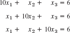
We consider the linear system

(Equations of this form arise in the numeric solution of PDEs and in spline interpolation.) We write the system in the form
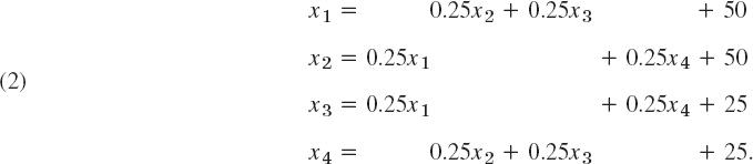
These equations are now used for iteration; that is, we start from a (possibly poor) approximation to the solution, say ![]() and compute from (2) a perhaps better approximation
and compute from (2) a perhaps better approximation
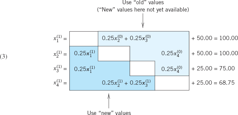
These equations (3) are obtained from (2) by substituting on the right the most recent approximation for each unknown. In fact, corresponding values replace previous ones as soon as they have been computed, so that in the second and third equations we use ![]() (not
(not ![]() ), and in the last equation of (3) we use
), and in the last equation of (3) we use ![]() and
and ![]() (not
(not ![]() and
and ![]() ). Using the same principle, we obtain in the next step
). Using the same principle, we obtain in the next step
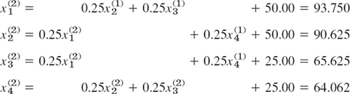
Further steps give the values
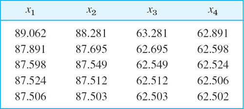
Hence convergence to the exact solution x1 = x2 = 87.5, x3 = x4 = 62.5 (verify!) seems rather fast.
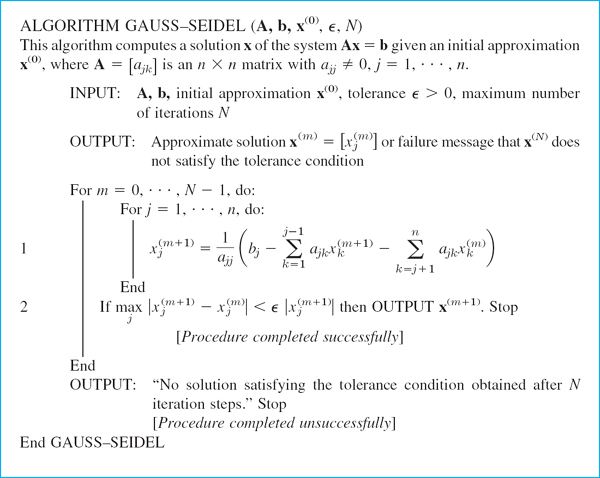
An algorithm for the Gauss–Seidel iteration is shown in Table 20.2. To obtain the algorithm, let us derive the general formulas for this iteration.
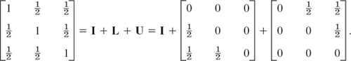
We assume that ajj = 1 for j = 1, …, n. (Note that this can be achieved if we can rearrange the equations so that no diagonal coefficient is zero; then we may divide each equation by the corresponding diagonal coefficient.) We now write
where I is the n × n unit matrix and L and U are, respectively, lower and upper triangular matrices with zero main diagonals. If we substitute (4) into Ax = b, we have
![]()
Taking Lx and Ux to the right, we obtain, since Ix = x,
![]()
Remembering from (3) in Example 1 that below the main diagonal we took “new” approximations and above the main diagonal “old” ones, we obtain from (5) the desired iteration formulas
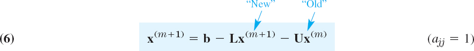
where ![]() is the mth approximation and
is the mth approximation and ![]() is the (m + 1)st approximation. In components this gives the formula in line 1 in Table 20.2. The matrix A must satisfy ajj ≠ 0 for all j. In Table 20.2 our assumption ajj = 1 is no longer required, but is automatically taken care of by the factor 1/ajj in line 1.
is the (m + 1)st approximation. In components this gives the formula in line 1 in Table 20.2. The matrix A must satisfy ajj ≠ 0 for all j. In Table 20.2 our assumption ajj = 1 is no longer required, but is automatically taken care of by the factor 1/ajj in line 1.
Table 20.2 Gauss–Seidel Iteration
Convergence and Matrix Norms
An iteration method for solving Ax = b is said to converge for an initial x(0) if the corresponding iterative sequence x(0), x(1), x(2), … converges to a solution of the given system. Convergence depends on the relation between x(m) and x(x+1). To get this relation for the Gauss–Seidel method, we use (6). We first have
![]()
and by multiplying by (I + L)−1 from the left,

The Gauss–Seidel iteration converges for every x(0) if and only if all the eigenvalues (Sec. 8.1) of the “iteration matrix” C = [cjk] have absolute value less than 1. (Proof in Ref. [E5], p. 191, listed in App. 1.)
CAUTION! If you want to get C, first divide the rows of A by ajj to have main diagonal 1, …, 1. If the spectral radius of C (= maximum of those absolute values) is small, then the convergence is rapid.
Sufficient Convergence Condition. A sufficient condition for convergence is
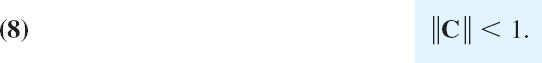
Here ||C|| is some matrix norm, such as

or the greatest of the sums of the |cjk| in a column of C

or the greatest of the sums of the |cjk| in a row of C

These are the most frequently used matrix norms in numerics.
In most cases the choice of one of these norms is a matter of computational convenience. However, the following example shows that sometimes one of these norms is preferable to the others.
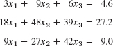
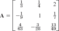
EXAMPLE 2 Test of Convergence of the Gauss–Seidel Iteration
Test whether the Gauss–Seidel iteration converges for the system
Solution. The decomposition (multiply the matrix by ![]() – why?) is
– why?) is
It shows that

We compute the Frobenius norm of C
![]()
and conclude from (8) that this Gauss–Seidel iteration converges. It is interesting that the other two norms would permit no conclusion, as you should verify. Of course, this points to the fact that (8) is sufficient for convergence rather than necessary.
Residual. Given a system Ax = b, the residual r of x with respect to this system is defined by

Clearly, r = 0 if and only if x is a solution. Hence r ≠ 0 for an approximate solution. In the Gauss–Seidel iteration, at each stage we modify or relax a component of an approximate solution in order to reduce a component of r to zero. Hence the Gauss–Seidel iteration belongs to a class of methods often called relaxation methods. More about the residual follows in the next section.
Jacobi Iteration
The Gauss–Seidel iteration is a method of successive corrections because for each component we successively replace an approximation of a component by a corresponding new approximation as soon as the latter has been computed. An iteration method is called a method of simultaneous corrections if no component of an approximation x(m) is used until all the components of x(m) have been computed. A method of this type is the Jacobi iteration, which is similar to the Gauss–Seidel iteration but involves not using improved values until a step has been completed and then replacing x(m) by x(m+1) at once, directly before the beginning of the next step. Hence if we write Ax = b (with ajj = 1 as before!) in the form x = b + (I − A)x, the Jacobi iteration in matrix notation is

This method converges for every choice of x(0) if and only if the spectral radius of I − A is less than 1. It has recently gained greater practical interest since on parallel processors all n equations can be solved simultaneously at each iteration step.
For Jacobi, see Sec. 10.3. For exercises, see the problem set.
- Verify the solution in Example 1 of the text.
- Show that for the system in Example 2 the Jacobi iteration diverges. Hint. Use eigenvalues.
- Verify the claim at the end of Example 2.
4–10 GAUSS–SEIDEL ITERATION
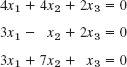
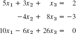
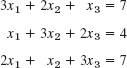
Do 5 steps, starting from x0 = [1 1 1]T and using 6S in the computation. Hint. Make sure that you solve each equation for the variable that has the largest coefficient (why?). Show the details.
- 4.

- 5.
- 6.

- 7.

- 8.
- 9.

- 10.

- 11. Apply the Gauss–Seidel iteration (3 steps) to the system in Prob. 5, starting from (a) 0, 0, 0 (b) 10, 10, 10. Compare and comment.
- 12. In Prob. 5, compute C (a) if you solve the first equation for x1, the second for x2, the third for x3, proving convergence; (b) if you nonsensically solve the third equation for x1, the first for x2, the second for x3, proving divergence.
- 13. CAS Experiment. Gauss–Seidel Iteration. (a) Write a program for Gauss–Seidel iteration.
- (b) Apply the program A(t)x = b, to starting from [0 0 0]T, where
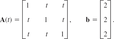
For t = 0.2, 0.5, 0.8, 0.9 determine the number of steps to obtain the exact solution to 6S and the corresponding spectral radius of C. Graph the number of steps and the spectral radius as functions of t and comment.
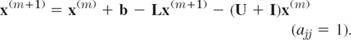
- (c) Successive overrelaxation (SOR). Show that by adding and subtracting x(m) on the right, formula (6) can be written
Anticipation of further corrections motivates the introduction of an overrelaxation factor ω > 1 to get the SOR formula for Gauss–Seidel
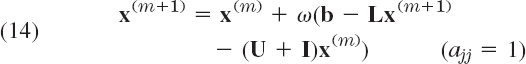
intended to give more rapid convergence. A recommended value is
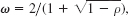 where ρ is the spectral radius of C in (7). Apply SOR to the matrix in (b) for t = 0.5 and 0.8 and notice the improvement of convergence. (Spectacular gains are made with larger systems.)
- (b) Apply the program A(t)x = b, to starting from [0 0 0]T, where
Do 5 steps, starting from x0 = [1 1 1]. Compare with the Gauss–Seidel iteration. Which of the two seems to converge faster? Show the details of your work.
- 14. The system in Prob. 4
- 15. The system in Prob. 9
- 16. The system in Prob. 10
- 17. Show convergence in Prob. 16 by verifying that I – A, where A is the matrix in Prob. 16 with the rows divided by the corresponding main diagonal entries, has the eigenvalues −0.519589 and 0.259795 ± 0.246603i.
18–20 NORMS
Compute the norms (9), (10), (11) for the following (square) matrices. Comment on the reasons for greater or smaller differences among the three numbers.
- 18. The matrix in Prob. 10
- 19. The matrix in Prob. 5
- 20.

20.4 Linear Systems: Ill-Conditioning, Norms
One does not need much experience to observe that some systems Ax = b are good, giving accurate solutions even under roundoff or coefficient inaccuracies, whereas others are bad, so that these inaccuracies affect the solution strongly. We want to see what is going on and whether or not we can “trust” a linear system. Let us first formulate the two relevant concepts (ill- and well-conditioned) for general numeric work and then turn to linear systems and matrices.
A computational problem is called ill-conditioned (or ill-posed) if “small” changes in the data (the input) cause “large” changes in the solution (the output). On the other hand, a problem is called well-conditioned (or well-posed) if “small” changes in the data cause only “small” changes in the solution.
These concepts are qualitative. We would certainly regard a magnification of inaccuracies by a factor 100 as “large,” but could debate where to draw the line between “large” and “small,” depending on the kind of problem and on our viewpoint. Double precision may sometimes help, but if data are measured inaccurately, one should attempt changing the mathematical setting of the problem to a well-conditioned one.
Let us now turn to linear systems. Figure 445 explains that ill-conditioning occurs if and only if the two equations give two nearly parallel lines, so that their intersection point (the solution of the system) moves substantially if we raise or lower a line just a little. For larger systems the situation is similar in principle, although geometry no longer helps. We shall see that we may regard ill-conditioning as an approach to singularity of the matrix.

Fig. 445. (a) Well-conditioned and (b) ill-conditioned linear system of two equations in two unknowns
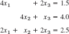
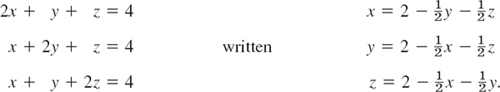
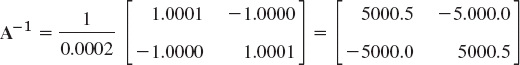
EXAMPLE 1 An Ill-Conditioned System
You may verify that the system
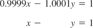
has the solution x = 0.5. y = −0.5, whereas the system

has the solution x = 0.5 + 5000.5![]() , y = −0.5 + 4999.5
, y = −0.5 + 4999.5![]() . This shows that the system is ill-conditioned because a change on the right of magnitude
. This shows that the system is ill-conditioned because a change on the right of magnitude ![]() produces a change in the solution of magnitude 5000
produces a change in the solution of magnitude 5000![]() , approximately. We see that the lines given by the equations have nearly the same slope.
, approximately. We see that the lines given by the equations have nearly the same slope.
Well-conditioning can be asserted if the main diagonal entries of A have large absolute values compared to those of the other entries. Similarly if A−1 and A have maximum entries of about the same absolute value.
Ill-conditioning is indicated if A−1 has entries of large absolute value compared to those of the solution (about 5000 in Example 1) and if poor approximate solutions may still produce small residuals.
Residual. The residual r of an approximate solution ![]() of Ax = b is defined as
of Ax = b is defined as

Now b = Ax, so that
![]()
Hence r is small if ![]() has high accuracy, but the converse may be false:
has high accuracy, but the converse may be false:
EXAMPLE 2 Inaccurate Approximate Solution with a Small Residual
The system

has the exact solution x1 = 1, x2 = 1. Can you see this by inspection? The very inaccurate approximation ![]() has the very small residual (to 4D)
has the very small residual (to 4D)

From this, a naive person might draw the false conclusion that the approximation should be accurate to 3 or 4 decimals.
Our result is probably unexpected, but we shall see that it has to do with the fact that the system is ill-conditioned.
Our goal is to show that ill-conditioning of a linear system and of its coefficient matrix A can be measured by a number, the condition number κ(A). Other measures for ill-conditioning have also been proposed, but κ(A) is probably the most widely used one. κ(A) is defined in terms of norm, a concept of great general interest throughout numerics (and in modern mathematics in general!). We shall reach our goal in three steps, discussing
- Vector norms
- Matrix norms
- Condition number κ of a square matrix
Vector Norms
A vector norm for column vectors x = [xj] with n components (n fixed) is a generalized length or distance. It is denoted by ||x|| and is defined by four properties of the usual length of vectors in three-dimensional space, namely,

If we use several norms, we label them by a subscript. Most important in connection with computations is the p-norm defined by
![]()
where p is a fixed number and p ![]() 1. In practice, one usually takes p = 1 or 2 and, as a third norm, ||x||∞ (the latter as defined below), that is,
1. In practice, one usually takes p = 1 or 2 and, as a third norm, ||x||∞ (the latter as defined below), that is,
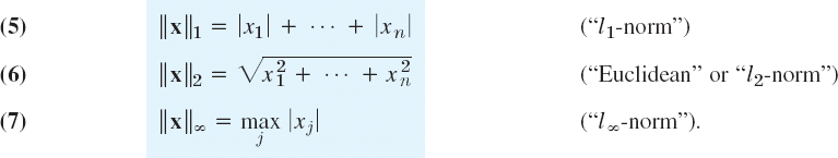
For n = 3 the l2-norm is the usual length of a vector in three-dimensional space. The l1-norm and l∞-norm are generally more convenient in computation. But all three norms are in common use.
In three-dimensional space, two points with position vectors x and ![]() have distance
have distance ![]() from each other. For a linear system Ax = b, this suggests that we take
from each other. For a linear system Ax = b, this suggests that we take ![]() as a measure of inaccuracy and call it the distance between an exact and an approximate solution, or the error of
as a measure of inaccuracy and call it the distance between an exact and an approximate solution, or the error of ![]() .
.
Matrix Norm
If A is an n × n matrix and x any vector with n components, then Ax is a vector with n components. We now take a vector norm and consider ||x|| and ||Ax||. One can prove (see Ref. [E17]. pp. 77, 92–93, listed in App. 1) that there is a number c (depending on A) such that
![]()
Let x ≠ 0. Then ||x|| > 0 by (3b) and division gives ||Ax||/||x|| ![]() c. We obtain the smallest possible c valid for all x (≠ 0) by taking the maximum on the left. This smallest c is called the matrix norm of A corresponding to the vector norm we picked and is denoted by ||A|| Thus
c. We obtain the smallest possible c valid for all x (≠ 0) by taking the maximum on the left. This smallest c is called the matrix norm of A corresponding to the vector norm we picked and is denoted by ||A|| Thus
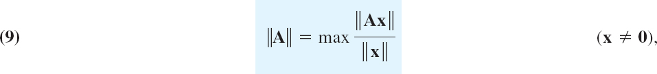
the maximum being taken over all x ≠ 0. Alternatively [see (c) in Team Project 24],
![]()
The maximum in (10) and thus also in (9) exists. And the name “matrix norm” is justified because ||A|| satisfies (3) with x and y replaced by A and B. (Proofs in Ref. [E17] pp. 77, 92–93.)
Note carefully that ||A|| depends on the vector norm that we selected. In particular, one can show that

By taking our best possible (our smallest) c = ||A|| we have from (8)
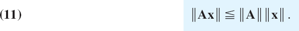
This is the formula we shall need. Formula (9) also implies for two n × n matrices (see Ref. [E17], p. 98)
![]()
See Refs. [E9] and [E17] for other useful formulas on norms.
Before we go on, let us do a simple illustrative computation.
Compute the matrix norms of the coefficient matrix A in Example 1 and of its inverse A−1, assuming that we use (a) the l1-vector norm, (b) the ![]() -vector norm.
-vector norm.
Solution. We use (4*), Sec. 7.8, for the inverse and then (10) and (11) in Sec. 20.3. Thus
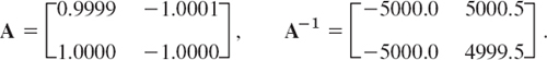
(a) The l1-vector norm gives the column “sum” norm (10), Sec. 20.3; from Column 2 we thus obtain ||A|| = |−1.0001| + |−1.0000| = 2.0001. Similarly, ||A−1|| = 10,000.
(b) The l∞-vector norm gives the row “sum” norm (11), Sec. 20.3; thus ||A|| = 2, ||A−1|| = 10000.5 from Row 1. We notice that ||A−1|| is surprisingly large, which makes the product ||A|| ||A−1|| large (20,001). We shall see below that this is typical of an ill-conditioned system.
Condition Number of a Matrix
We are now ready to introduce the key concept in our discussion of ill-conditioning, the condition number κ(A) of a (nonsingular) square matrix A, defined by

The role of the condition number is seen from the following theorem.
A linear system of equations Ax = b and its matrix A whose condition number (13) is small are well-conditioned. A large condition number indicates ill-conditioning.
PROOF
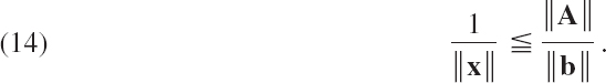
b = Ax and (11) give ||b|| ![]() ||A|| ||x||. Let b ≠ 0 and x ≠ 0. Then division by ||b|| ||x|| gives
||A|| ||x||. Let b ≠ 0 and x ≠ 0. Then division by ||b|| ||x|| gives
Multiplying (2) ![]() by A−1 from the left and interchanging sides, we have
by A−1 from the left and interchanging sides, we have ![]() Now (11) with A−1 and r instead of A and x yields
Now (11) with A−1 and r instead of A and x yields
![]()
Division by ||x|| [note that ||x|| ≠ 0 by (3b)] and use of (14) finally gives

Hence if κ(A) is small, a small ||r||/||b|| implies a small relative error ![]() , so that the system is well-conditioned. However, this does not hold if κ(A) is large; then a small ||r||/||b|| does not necessarily imply a small relative error
, so that the system is well-conditioned. However, this does not hold if κ(A) is large; then a small ||r||/||b|| does not necessarily imply a small relative error ![]() .
.
EXAMPLE 5 Condition Numbers. Gauss–Seidel Iteration
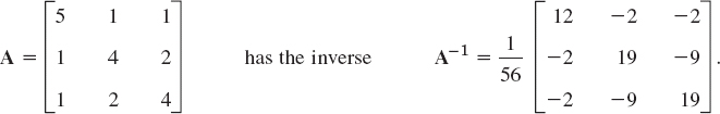
Since A is symmetric, (10) and (11) in Sec. 20.3 give the same condition number
![]()
We see that a linear system Ax = b with this A is well-conditioned.
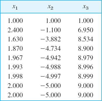
For instance, if b = [14 0 28]T, the Gauss algorithm gives the solution x = [2 −5 9]T, (confirm this). Since the main diagonal entries of A are relatively large, we can expect reasonably good convergence of the Gauss–Seidel iteration. Indeed, starting from, say, x0 = [1 1 1]T, we obtain the first 8 steps (3D values)
EXAMPLE 6 Ill-Conditioned Linear System
Example 4 gives by (10) or (11), Sec. 20.3, for the matrix in Example 1 the very large condition number κ(A) = 2.0001 · 10000 = 2 · 10000.5 = 200001. This confirms that the system is very ill-conditioned.
Similarly in Example 2, where by (4*), Sec. 7.8 and 6D-computation,
so that (10), Sec. 20.3, gives a very large κ(A), explaining the surprising result in Example 2,
![]()
In practice, A−1 will not be known, so that in computing the condition number κ(A), one must estimate ||A−1||. A method for this (proposed in 1979) is explained in Ref. [E9] listed in App. 1.
Inaccurate Matrix Entries. κ(A) can be used for estimating the effect δx of an inaccuracy δA of A (errors of measurements of the ajk, for instance). Instead of Ax = b we then have
![]()
Multiplying out and subtracting Ax = b on both sides, we obtain
![]()
Multiplication by A−1 from the left and taking the second term to the right gives
![]()
Applying (11) with A−1 and vector δA(x + δx) instead of A and x, we get
![]()
Applying (11) on the right, with δA and x − δx instead of A and x, we obtain
![]()
Now ||A−1|| = κ(A)/||A|| by the definition of κ(A), so that division by ||x + δx|| shows that the relative inaccuracy of x is related to that of A via the condition number by the inequality
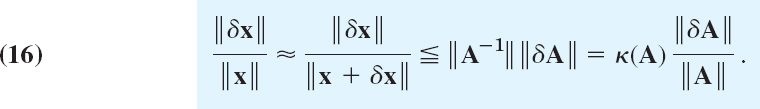
Conclusion. If the system is well-conditioned, small inaccuracies ||δA||/||A|| can have only a small effect on the solution. However, in the case of ill-conditioning, if ||δA||/||A|| is small, ||δx||/||x|| may be large.
Inaccurate Right Side. You may show that, similarly, when A is accurate, an inaccuracy of δb of b causes an inaccuracy δx satisfying

Hence ||δx||/||x|| must remain relatively small whenever κ(A) is small.
EXAMPLE 7 Inaccuracies. Bounds (16) and (17)
If each of the nine entries of A in Example 5 is measured with an inaccuracy of 0.1, then ||δA|| = 9 · 0.1 and (16) gives

By experimentation you will find that the actual inaccuracy ||δx|| is only about 30% of the bound 5.14. This is typical.
Similarly, if δb = [0.1 0.1]T, then ||δb|| = 0.3 and ||b|| = 42 in Example 5, so that (17) gives
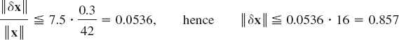
but this bound is again much greater than the actual inaccuracy, which is about 0.15.
Further Comments on Condition Numbers. The following additional explanations may be helpful.
1. There is no sharp dividing line between “well-conditioned” and “ill-conditioned,” but generally the situation will get worse as we go from systems with small κ(A) to systems with larger κ(A). Now always κ(A) ![]() 1, so that values of 10 or 20 or so give no reason for concern, whereas κ(A) = 100, say, calls for caution, and systems such as those in Examples 1 and 2 are extremely ill-conditioned.
1, so that values of 10 or 20 or so give no reason for concern, whereas κ(A) = 100, say, calls for caution, and systems such as those in Examples 1 and 2 are extremely ill-conditioned.
2. If κ(A) is large (or small) in one norm, it will be large (or small, respectively) in any other norm. See Example 5.
3. The literature on ill-conditioning is extensive. For an introduction to it, see [E9].
This is the end of our discussion of numerics for solving linear systems. In the next section we consider curve fitting, an important area in which solutions are obtained from linear systems.
1–6 VECTOR NORMS
Compute the norms (5), (6), (7). Compute a corresponding unit vector (vector of norm 1) with respect to the l∞-norm.
- [1 −3 8 0 −6 0]
- [4 −1 8]
- [0.2 0.6 −2.1 3.0]
- [k2, 4k, k3], k > 4
- [1 1 1 1 1]
- [0 0 0 1 0]
- For what x = [a b c] will ||x||1 = ||x||2?
- Show that ||x||∞
 ||x||2 ||x||1.
[9–16] MATRIX NORMS, CONDITION NUMBERS
Compute the matrix norm and the condition number corresponding to the l1-vector norm.
- 9.

- 10.

- 11.

- 12.

- 13.

- 14.

- 15.
- 16.
- 17. Verify (11) for x = [3 15 −4]T taken with the l∞-norma and the matrix in Prob. 13.
- 18. Verify (12) for the matrices in Probs. 9 and 10.
[19–20] ILL-CONDITIONED SYSTEMS
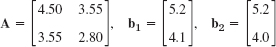
Solve Ax = b1, Ax = b2. Compare the solutions and comment. Compute the condition number of A.
- 19.
- 20.

- 21. Residual. For Ax = b1 in Prob. 19 guess what the residual of
 , very poorly approximating [−2 4]T, might be. Then calculate and comment.
 - 22. Show that κ(A)
 1 for the matrix norms (10), (11), Sec. 20.3, and
  for the Frobenius norm (9), Sec. 20.3.
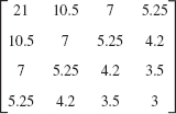
 - 23. CAS EXPERIMENT. Hilbert Matrices. The 3 × 3 Hilbert matrix is
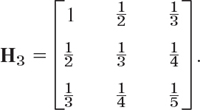
The n × n Hilbert matrix is Hn = [hjk], where hjk = 1/(j + k − 1). (Similar matrices occur in curve fitting by least squares.) Compute the condition number κ(Hn) for the matrix norm corresponding to the l∞-(or l1-) vector norm, for n = 2, 3, …, 6 (or further if you wish). Try to find a formula that gives reasonable approximate values of these rapidly growing numbers.
Solve a few linear systems of your choice, involving an Hn.
- 24. TEAM PROJECT. Norms. (a) Vector norms in our text are equivalent, that is, they are related by double inequalities; for instance,

Hence if for some x, one norm is large (or small), the other norm must also be large (or small). Thus in many investigations the particular choice of a norm is not essential. Prove (18).
- (b) The Cauchy–Schwarz inequality is

It is very important. (Proof in Ref. [GenRef7] listed in App. 1.) Use it to prove


- (c) Formula (10) is often more practical than (9). Derive (10) from (9).
- (d) Matrix norms. Illustrate (11) with examples. Give examples of (12) with equality as well as with strict inequality. Prove that the matrix norms (10), (11) in Sec. 20.3 satisfy the axioms of a norm

- (b) The Cauchy–Schwarz inequality is
- 25. WRITING PROJECT. Norms and Their Use in This Section. Make a list of the most important of the many ideas covered in this section and write a two-page report on them.
20.5 Least Squares Method
Having discussed numerics for linear systems, we now turn to an important application, curve fitting, in which the solutions are obtained from linear systems.
In curve fitting we are given n points (pairs of numbers) (x1, y1), …, (xn, yn) and we want to determine a function f(x) such that
![]()
approximately. The type of function (for example, polynomials, exponential functions, sine and cosine functions) may be suggested by the nature of the problem (the underlying physical law, for instance), and in many cases a polynomial of a certain degree will be appropriate.
Let us begin with a motivation.
If we require strict equality f(x1) = y1, …,f(xn) = yn and use polynomials of sufficiently high degree, we may apply one of the methods discussed in Sec. 19.3 in connection with interpolation. However, in certain situations this would not be the appropriate solution of the actual problem. For instance, to the four points
![]()
there corresponds the interpolation polynomial f(x) = x3 − x + 2 (Fig. 446), but if we graph the points, we see that they lie nearly on a straight line. Hence if these values are obtained in an experiment and thus involve an experimental error, and if the nature of the experiment suggests a linear relation, we better fit a straight line through the points (Fig. 446). Such a line may be useful for predicting values to be expected for other values of x. A widely used principle for fitting straight lines is the method of least squares by Gauss and Legendre. In the present situation it may be formulated as follows.
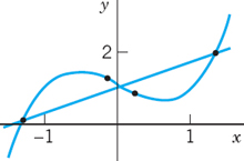
Fig. 446. Approximate fitting of a straight line
Method of Least Squares. The straight line
![]()
should be fitted through the given points (x1, y1), …, (xn, yn) so that the sum of the squares of the distances of those points from the straight line is minimum, where the distance is measured in the vertical direction (the y-direction).
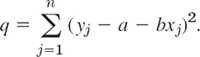
The point on the line with abscissa xj has the ordinate a + bxj. Hence its distance from (xj, yj) is |yj − a − bxj| (Fig. 447) and that sum of squares is
q depends on a and b. A necessary condition for q to be minimum is
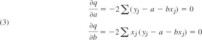
(where we sum over j from 1 to n). Dividing by 2, writing each sum as three sums, and taking one of them to the right, we obtain the result
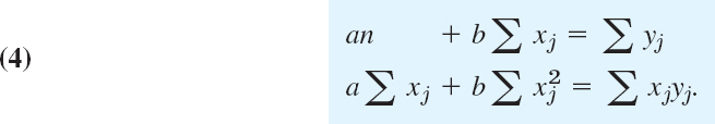
These equations are called the normal equations of our problem.
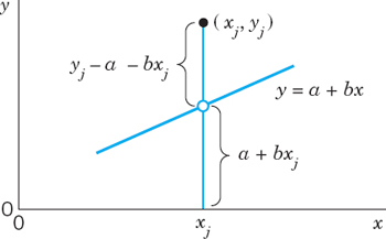
Fig. 447. Vetrical distance of a point (xj, yj) from a straight line y = a + bx
Using the method of least squares, fit a straight line to the four points given in formula (1).
Solution. We obtain
![]()
Hence the normal equations are

The solution (rounded to 4D) is a = 0.9601, b = 0.6670, and we obtain the straight line (Fig. 446)
![]()
Curve Fitting by Polynomials of Degree m
Our method of curve fitting can be generalized from a polynomial y = a + bx to a polynomial of degree m
![]()
where m ![]() n − 1. Then q takes the form
n − 1. Then q takes the form

and depends on m + 1 parameters b0, …,bm. Instead of (3) we then have m + 1 conditions

which give a system of m + 1 normal equations.
In the case of a quadratic polynomial
![]()
the normal equations are (summation from 1 to n)
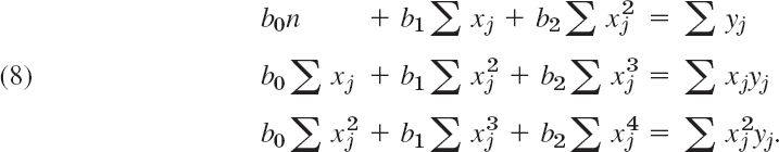
The derivation of (8) is left to the reader.
EXAMPLE 2 Quadratic Parabola by Least Squares
Fit a parabola through the data (0, 5), (2, 4), (4, 1), (6, 6), (8, 7).
Solution. For the normal equations we need n = 5, Σxj = 20, ![]() Σyj = 23,
Σyj = 23, ![]() Hence these equations are
Hence these equations are

Solving them we obtain the quadratic least squares parabola (Fig. 448)
![]()
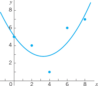
Fig. 448. Least squares parabola in Example 2
For a general polynomial (5) the normal equations form a linear system of equations in the unknowns b0, … bm. When its matrix M is nonsingular, we can solve the system by Cholesky's method (Sec. 20.2) because then M is positive definite (and symmetric). When the equations are nearly linearly dependent, the normal equations may become ill-conditioned and should be replaced by other methods; see [E5], Sec. 5.7, listed in App. 1.
The least squares method also plays a role in statistics (see Sec. 25.9).
[1–6] FITTING A STRAIGHT LINE
Fit a straight line to the given points (x, y) by least squares. Show the details. Check your result by sketching the points and the line. Judge the goodness of fit.
- (0, 2), (2, 0), (3, −2), (5, −3)
- How does the line in Prob. 1 change if you add a point far above it, say, (1, 3)? Guess first.
- (0, 1.8), (1, 1.6), (2, 1.1), (3, 1.5), (4, 2.3)
- Hooke's law F = ks. Estimate the spring modulus k from the force F [lb] and the elongation s [cm], where (F, s) = (1, 0.3), (2, 0.7), (4, 1.3), (6, 1.9), (10, 3.2), (20, 6.3).
- Average speed. Estimate the average speed vav of a car traveling according to s = v · t [km] (s = distance traveled, t [hr] = time) from (t, s) = (9, 140), (10, 220), (11, 310), (12, 410).
- Ohm's law U = Ri. Estimate R from (i, U) = (2, 104), (4, 206), (6, 314), (10, 530).
- Derive the normal equations (8).
[8–11] FITTING A QUADRATIC PARABOLA
Fit a parabola (7) to the points (x, y). Check by sketching.
- 8. (−1, 5), (1, 3), (2, 4), (3, 8)
- 9. (2, −3), (3, 0), (5, 1), (6, 0) (7, −2)
- 10. t[hr] = Worker's time on duty, y[sec] = His/her reaction time, (t, y) = (1, 2.0), (2, 1.78), (3, 1.90), (4, 2.35), (5, 2.70)
- 11. The data in Prob. 3. Plot the points, the line, and the parabola jointly. Compare and comment.
- 12. Cubic parabola. Derive the formula for the normal equations of a cubic least squares parabola.
- 13. Fit curves (2) and (7) and a cubic parabola by least squares to (x, y) = (−2, −30), (−1, −4), (0, 4), (1, 4), (2, 22), (3, 68). Graph these curves and the points on common axes. Comment on the goodness of fit.
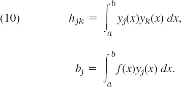
- 14. TEAM PROJECT. The least squares approximation of a function f(x) on an interval a x b by a function

where y0(x), …,ym(x) are given functions, requires the determination of the coefficients a0, …,am such that
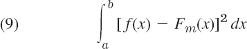
becomes minimum. This integral is denoted by ||f − Fm||2, and ||f − Fm|| is called the L2-norm of f − Fm (L suggesting Lebesgue5). A necessary condition for that minimum is given by ∂||f − Fm||2/∂aj = 0, j = 0, …,m [the analog of (6)]. (a) Show that this leads to m + 1 normal equations (j = 0, …,m)
- (b) Polynomial. What form does (10) take if Fm(x) = a0 + a1x + … + amxm? What is the coefficient matrix of (10) in this case when the interval is 0 x 1?
- (c) Orthogonal functions. What are the solutions of (10) if y0(x), …, ym(x) are orthogonal on the interval a x b? (For the definition, see Sec. 11.5. See also Sec. 11.6.)
- (b) Polynomial. What form does (10) take if Fm(x) = a0 + a1x + … + amxm? What is the coefficient matrix of (10) in this case when the interval is 0
- 15. CAS EXPERIMENT. Least Squares versus Interpolation. For the given data and for data of your choice find the interpolation polynomial and the least squares approximations (linear, quadratic, etc.). Compare and comment.
(a) (−2, 0), (−1, 0), (0, 1), (1, 0), (2, 0)
(b) (−4, 0), (−3, 0), (−2, 0), (−1, 0), (0, 1), (1, 0), (2, 0), (3, 0), (4, 0)
(c) Choose five points on a straight line, e.g., (0, 0), (1, 1), …, (4, 4). Move one point 1 unit upward and find the quadratic least squares polynomial. Do this for each point. Graph the five polynomials on common axes. Which of the five motions has the greatest effect?
20.6 Matrix Eigenvalue Problems: Introduction
We now come to the second part of our chapter on numeric linear algebra. In the first part of this chapter we discussed methods of solving systems of linear equations, which included Gauss elimination with backward substitution. This method is known as a direct method since it gives solutions after a prescribed amount of computation. The Gauss method was modified by Doolittle's method, Crout's method, and Cholesky's method, each requiring fewer arithmetic operations than Gauss. Finally we presented indirect methods of solving systems of linear equations, that is, the Gauss–Seidel method and the Jacobi iteration. The indirect methods require an undetermined number of iterations. That number depends on how far we start from the true solution and what degree of accuracy we require. Moreover, depending on the problem, convergence may be fast or slow or our computation cycle might not even converge. This led to the concepts of ill-conditioned problems and condition numbers that help us gain some control over difficulties inherent in numerics.
The second part of this chapter deals with some of the most important ideas and numeric methods for matrix eigenvalue problems. This very extensive part of numeric linear algebra is of great practical importance, with much research going on, and hundreds, if not thousands, of papers published in various mathematical journals (see the references in [E8], [E9], [E11], [E29]). We begin with the concepts and general results we shall need in explaining and applying numeric methods for eigenvalue problems. (For typical models of eigenvalue problems see Chap. 8.)
An eigenvalue or characteristic value (or latent root) of a given n × n matrix A = [ajk] is a real or complex number λ such that the vector equation

has a nontrivial solution, that is, a solution x ≠ 0, which is then called an eigenvector or characteristic vector of A corresponding to that eigenvalue λ. The set of all eigenvalues of A is called the spectrum of A. Equation (1) can be written
![]()
where I is the n × n unit matrix. This homogeneous system has a nontrivial solution if and only if the characteristic determinant det (A − λI) is 0 (see Theorem 2 in Sec. 7.5). This gives (see Sec. 8.1)

Developing the characteristic determinant, we obtain the characteristic polynomial of A, which is of degree n in λ. Hence A has at least one and at most n numerically different eigenvalues. If A is real, so are the coefficients of the characteristic polynomial. By familiar algebra it follows that then the roots (the eigenvalues of A) are real or complex conjugates in pairs.
To give you some orientation of the underlying approaches of numerics for eigenvalue problems, note the following. For large or very large matrices it may be very difficult to determine the eigenvalues, since, in general, it is difficult to find the roots of characteristic polynomials of higher degrees. We will discuss different numeric methods for finding eigenvalues that achieve different results. Some methods, such as in Sec. 20.7, will give us only regions in which complex eigenvalues lie (Geschgorin's method) or the intervals in which the largest and smallest real eigenvalue lie (Collatz method). Other methods compute all eigenvalues, such as the Householder tridiagonalization method and the QR-method in Sec. 20.9.
To continue our discussion, we shall usually denote the eigenvalues of A by
with the understanding that some (or all) of them may be equal.
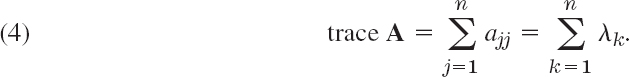
The sum of these n eigenvalues equals the sum of the entries on the main diagonal of A, called the trace of A; thus
Also, the product of the eigenvalues equals the determinant of A,
![]()
Both formulas follow from the product representation of the characteristic polynomial, which we denote by f(λ),
![]()
If we take equal factors together and denote the numerically distinct eigenvalues of A by λ1, …λr(r ![]() n), then the product becomes
n), then the product becomes
![]()
The exponent mj is called the algebraic multiplicity of λj. The maximum number of linearly independent eigenvectors corresponding to λj is called the geometric multiplicity of λj. It is equal to or smaller than mj.
A subspace S of Rn or Cn (if A is complex) is called an invariant subspace of A if for every v in S the vector Av is also in S. Eigenspaces of A (spaces of eigenvectors; Sec. 8.1) are important invariant subspaces of A.
An n × n matrix B is called similar to A if there is a nonsingular n × n matrix T such that

Similarity is important for the following reason.
Similar matrices have the same eigenvalues. If x is an eigenvector of A, then y = T−1x is an eigenvector of B in (7) corresponding to the same eigenvalue. (Proof in Sec. 8.4.)
Another theorem that has various applications in numerics is as follows.
If A has the eigenvalues λ1, …, λn, then A − kI with arbitrary k has the eigenvalues λ1 − k, …,λn − k.
This theorem is a special case of the following spectral mapping theorem.
If λ is an eigenvalue of A, then
![]()
is an eigenvalue of the polynomial matrix
![]()

The eigenvalues of important special matrices can be characterized as follows.
The eigenvalues of Hermitian matrices ( i.e., ![]() ), hence of real symmetric matrices ( i.e., AT = A), are real. The eigenvalues of skew-Hermitian matrices (i.e.,
), hence of real symmetric matrices ( i.e., AT = A), are real. The eigenvalues of skew-Hermitian matrices (i.e., ![]() ), hence of real skew-symmetric matrices (i.e., AT = −A), are pure imaginary or 0. The eigenvalues of unitary matrices (i.e.,
), hence of real skew-symmetric matrices (i.e., AT = −A), are pure imaginary or 0. The eigenvalues of unitary matrices (i.e., ![]() ), hence of orthogonal matrices (i.e., AT = A−1), have absolute value 1. (Proofs in Secs. 8.3 and 8.5.)
), hence of orthogonal matrices (i.e., AT = A−1), have absolute value 1. (Proofs in Secs. 8.3 and 8.5.)
The choice of a numeric method for matrix eigenvalue problems depends essentially on two circumstances, on the kind of matrix (real symmetric, real general, complex, sparse, or full) and on the kind of information to be obtained, that is, whether one wants to know all eigenvalues or merely specific ones, for instance, the largest eigenvalue, whether eigenvalues and eigenvectors are wanted, and so on. It is clear that we cannot enter into a systematic discussion of all these and further possibilities that arise in practice, but we shall concentrate on some basic aspects and methods that will give us a general understanding of this fascinating field.
20.7 Inclusion of Matrix Eigenvalues
The whole of numerics for matrix eigenvalues is motivated by the fact that, except for a few trivial cases, we cannot determine eigenvalues exactly by a finite process because these values are the roots of a polynomial of n th degree. Hence we must mainly use iteration.
In this section we state a few general theorems that give approximations and error bounds for eigenvalues. Our matrices will continue to be real (except in formula (5) below), but since (nonsymmetric) matrices may have complex eigenvalues, complex numbers will play a (very modest) role in this section.
The important theorem by Gerschgorin gives a region consisting of closed circular disks in the complex plane and including all the eigenvalues of a given matrix. Indeed, for each j = 1, …,n the inequality (1) in the theorem determines a closed circular disk in the complex λ-plane with center ajj and radius given by the right side of (1); and Theorem 1 states that each of the eigenvalues of A lies in one of these n disks.
THEOREM 1 Gerschgorin's Therorem6
Let λ be an eigenvalue of an arbitrary n × n matrix A = [ajk]. Then for some integer j (1 ![]() j
j ![]() n) we have
n) we have
![]()
Let x be an eigenvector corresponding to an eigenvalue λ of A. Then
![]()
Let xj be a component of x that is largest in absolute value. Then we have |xm/xj| ![]() 1 for m = 1, …,n. The vector equation (2) is equivalent to a system of n equations for the n components of the vectors on both sides. The jth of these n equations with j as just indicated is
1 for m = 1, …,n. The vector equation (2) is equivalent to a system of n equations for the n components of the vectors on both sides. The jth of these n equations with j as just indicated is
![]()
Division by xj (which cannot be zero; why?) and reshuffling terms gives

By taking absolute values on both sides of this equation, applying the triangle inequality |a + b|![]() |a| + |b| (where a and b are any complex numbers), and observing that because of the choice of j (which is crucial!), |x1/xj|
|a| + |b| (where a and b are any complex numbers), and observing that because of the choice of j (which is crucial!), |x1/xj| ![]() 1, …,|xn/xj
1, …,|xn/xj![]() 1 we obtain (1), and the theorem is proved.
1 we obtain (1), and the theorem is proved.
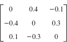
EXAMPLE 1 Gerschgorin's Theorem
For the eigenvalues of the matrix
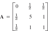
we get the Gerschgorin disks (Fig. 449)
![]()
The centers are the main diagonal entries of A. These would be the eigenvalues of A if A were diagonal. We can take these values as crude approximations of the unknown eigenvalues (3D-values) λ1 = −0.209, λ2 = 5.305, λ3 = 0.904 (verify this); then the radii of the disks are corresponding error bounds.
Since A is symmetric, it follows from Theorem 5, Sec. 20.6, that the spectrum of A must actually lie in the intervals [−1, 2.5] and [3.5, 6.5].
It is interesting that here the Gerschgorin disks form two disjoint sets, namely, D1 ∪ D3 which contains two eigenvalues, and D2, which contains one eigenvalue. This is typical, as the following theorem shows.

Fig. 449. Gerschgorin disks in Example 1
THEOREM 2 Extension of Gerschgorin's Theorem
If p Gerschgorin disks form a set S that is disjoint from the n − p other disks of a given matrix A, then S contains precisely p eigenvalues of A (each counted with its algebraic multiplicity, as defined in Sec. 20.6).
Idea of Proof. Set A = B + C, where B is the diagonal matrix with entries ajj, and apply Theorem 1 to At = B + tC with real t growing from 0 to 1.
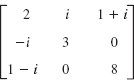
EXAMPLE 2 Another Application of Gerschgorin's Theorem. Similarity
Suppose that we have diagonalized a matrix by some numeric method that left us with some off-diagonal entries of size 10−5 say,
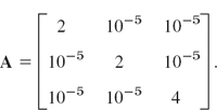
What can we conclude about deviations of the eigenvalues from the main diagonal entries?
Solution. By Theorem 2, one eigenvalue must lie in the disk of radius 2 · 10−5 centered at 4 and two eigenvalues (or an eigenvalue of algebraic multiplicity 2) in the disk of radius 2 · 10−5 centered at 2. Actually, since the matrix is symmetric, these eigenvalues must lie in the intersections of these disks and the real axis, by Theorem 5 in Sec. 20.6.
We show how an isolated disk can always be reduced in size by a similarity transformation. The matrix
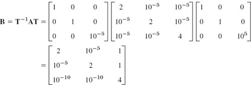
is similar to A. Hence by Theorem 2, Sec. 20.6, it has the same eigenvalues as A. From Row 3 we get the smaller disk of radius 2 · 10−10. Note that the other disks got bigger, approximately by a factor of 105. And in choosing T we have to watch that the new disks do not overlap with the disk whose size we want to decrease.
For further interesting facts, see the book [E28].
By definition, a diagonally dominant matrix A = [ajk] is an n × n matrix such that

where we sum over all off-diagonal entries in Row j. The matrix is said to be strictly diagonally dominant if > in (3) for all j. Use Theorem 1 to prove the following basic property.
Further Inclusion Theorems
An inclusion theorem is a theorem that specifies a set which contains at least one eigenvalue of a given matrix. Thus, Theorems 1 and 2 are inclusion theorems; they even include the whole spectrum. We now discuss some famous theorems that yield further inclusions of eigenvalues. We state the first two of them without proofs (which would exceed the level of this book).
THEOREM 4 Schur's Theorem7
Let A = [ajk] be a n × n matrix. Then for each of its eigenvalues λ1, …, λn,

In (4) the second equality sign holds if and only if A is such that
![]()
Matrices that satisfy (5) are called normal matrices. It is not difficult to see that Hermitian, skew-Hermitian, and unitary matrices are normal, and so are real symmetric, skew-symmetric, and orthogonal matrices.
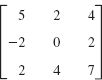
EXAMPLE 3 Bounds for Eigenvalues Obtained from Schur's Inequality
For the matrix

we obtain from Schur's inequality ![]() . You may verify that the eigenvalues are 30, 25, and 20. Thus 302 + 252 + 202 = 1925 < 1949 in fact, A is not normal.
. You may verify that the eigenvalues are 30, 25, and 20. Thus 302 + 252 + 202 = 1925 < 1949 in fact, A is not normal.
The preceding theorems are valid for every real or complex square matrix. Other theorems hold for special classes of matrices only. Famous is the following one, which has various applications, for instance, in economics.
THEOREM 5 Perron's Theorem8
Let A be a real n × n matrix whose entries are all positive. Then A has a positive real eigenvalue λ = ρ of multiplicity 1. The corresponding eigenvector can be chosen with all components positive. (The other eigenvalues are less than in absolute value.)
For a proof see Ref. [B3], vol. II, pp. 53–62. The theorem also holds for matrices with nonnegative real entries (“Perron–Frobenius Theorem”8) provided A is irreducible, that is, it cannot be brought to the following form by interchanging rows and columns; here B and F are square and 0 is a zero matrix.

Perron's theorem has various applications, for instance, in economics. It is interesting that one can obtain from it a theorem that gives a numeric algorithm:
THEOREM 6 Collatz Inclusion Theorem9
Let A = [ajk] be a real matrix n × n whose elements are all positive. Let x be any real vector whose components x1, …, xn are positive, and let y1, …, yn be the components of the vector y = Ax. Then the closed interval on the real axis bounded by the smallest and the largest of the n quotients qj = yj/xj contains at least one eigenvalue of A.
PROOF
We have Ax = y or
![]()
The transpose AT satisfies the conditions of Theorem 5. Hence AT has a positive eigenvalue λ and, corresponding to this eigenvalue, an eigenvector u whose components uj are all positive. Thus ATu = λu and by taking the transpose we obtain uTA = λuT. From this and (6) we have
![]()
or written out
Since all the components uj are positive, it follows that

Since A and AT have the same eigenvalues, λ is an eigenvalue of A, and from (7) the statement of the theorem follows.
EXAMPLE 4 Bounds for Eigenvalues from Collatz's Theorem. Iteration
For a given matrix A with positive entries we choose an x = x0 and iterate, that is, we compute x1 = Ax0, x2 = Ax1, …,x20 = Ax19. In each step, taking x = xj and y = Axj = xj+1 we compute an inclusion interval by Collatz's theorem. This gives (6S)
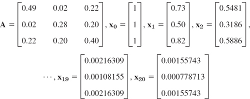
and the intervals 0.5 ![]() λ
λ ![]() 0.82, 0.3186/0.50 = 0.6372
0.82, 0.3186/0.50 = 0.6372 ![]() λ
λ ![]() 0.5481/0.73 = 0.750822, etc. These intervals have length
0.5481/0.73 = 0.750822, etc. These intervals have length

Using the characteristic polynomial, you may verify that the eigenvalues of A are 0.72, 0.36, 0.09, so that those intervals include the largest eigenvalue, 0.72. Their lengths decreased with j, so that the iteration was worthwhile. The reason will appear in the next section, where we discuss an iteration method for eigenvalues.
1–6 GERSCHGORIN DISKS
Find and sketch disks or intervals that contain the eigenvalues. If you have a CAS, find the spectrum and compare.


- Similarity. In Prob. 2, find T−TAT such that the radius of the Gerschgorin circle with center 5 is reduced by a factor 1/100.
- By what integer factor can you at most reduce the Gerschgorin circle with center 3 in Prob. 6?
- If a symmetric n × n matrix A = [ajk] has been diagonalized except for small off-diagonal entries of size 10−5, what can you say about the eigenvalues?
- Optimality of Gerschgorin disks. Illustrate with a 2 × 2 matrix that an eigenvalue may very well lie on a Gerschgorin circle, so that Gerschgorin disks can generally not be replaced with smaller disks without losing the inclusion property.
- Spectral radius ρ(A) Using Theorem 1, show that ρ(A) cannot be greater than the row sum norm of A.
12–16 SPECTRAL RADIUS
Use (4) to obtain an upper bound for the spectral radius:
- 12. In Prob. 4
- 13. In Prob. 1
- 14. In Prob. 6
- 15. In Prob. 3
- 16. In Prob. 5
- 17. Verify that the matrix in Prob. 5 is normal.
- 18. Normal matrices. Show that Hermitian, skew-Hermitian, and unitary matrices (hence real symmetric, skew-symmetric, and orthogonal matrices) are normal. Why is this of practical interest?
- 19. Prove Theorem 3 by using Theorem 1.
- 20. Extended Gerschgorin theorem. Prove Theorem 2. Hint. Let A = B + C, B = diag (ajj), At = B + tC, and let t increase continuously from 0 to 1.
20.8 Power Method for Eigenvalues
A simple standard procedure for computing approximate values of the eigenvalues of an n × n matrix A = [ajk] is the power method. In this method we start from any vector x0 (≠ 0) with n components and compute successively
![]()
For simplifying notation, we denote Xs−1 by x and xs by y, so that y = Ax.
The method applies to any n × n matrix A that has a dominant eigenvalue (a λ such that |λ| is greater than the absolute values of the other eigenvalues). If A is symmetric, it also gives the error bound (2), in addition to the approximation (1).
THEOREM 1 Power Method, Error Bounds
Let A be an n × n real symmetric matrix. Let x (≠0) be any real vector with n components. Furthermore, let
![]()
Then the quotient

is an approximation for an eigenvalue λ of A (usually that which is greatest in absolute value, but no general statements are possible).
Furthermore, if we set q = λ − ε, so that ε is the error of q, then
PROOF
δ2 denotes the radicand in (2). Since m1 = qm0 by (1), we have
(3) ![]()
Since A is real symmetric, it has an orthogonal set of n real unit eigenvectors z1, …,zn corresponding to the eigenvalues λ1, …, λn, respectively (some of which may be equal). (Proof in Ref. [B3], vol. 1, pp. 270–272, listed in App. 1.) Then x has a representation of the form
![]()
Now Az1 = λ1z1, etc., and we obtain
![]()
and, since the zj are orthogonal unit vectors,
![]()
It follows that in (3),
![]()
Since the zj are orthogonal unit vectors, we thus obtain from (3)
![]()
Now let λc be an eigenvalue of A to which q is closest, where c suggests “closest.” Then (λc − q)2 ![]() (λj − q)2 for j = 1, …,n. From this and (5) we obtain the inequality
(λj − q)2 for j = 1, …,n. From this and (5) we obtain the inequality
![]()
Dividing by m0 taking square roots, and recalling the meaning of δ2 gives
This shows that δ is a bound for the error ε of the approximation q of an eigenvalue of A and completes the proof.
The main advantage of the method is its simplicity. And it can handle sparse matrices too large to store as a full square array. Its disadvantage is its possibly slow convergence. From the proof of Theorem 1 we see that the speed of convergence depends on the ratio of the dominant eigenvalue to the next in absolute value (2:1 in Example 1, below).
If we want a convergent sequence of eigenvectors, then at the beginning of each step we scale the vector, say, by dividing its components by an absolutely largest one, as in Example 1, as follows.
EXAMPLE 1 Application of Theorem 1. Scaling
For the symmetric matrix A in Example 4, Sec. 20.7, and x0 = [1 1 1]T we obtain from (1) and (2) and the indicated scaling
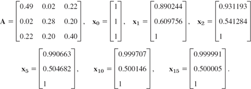
Here Ax0 = [0.73 0.5 0.82]T, scaled to x1 = [0.73/0.82 0.5/0.82 1]T, etc. The dominant eigenvalue is 0.72, an eigenvector [1 0.5 1]T. The corresponding q and δ are computed each time before the next scaling. Thus in the first step,
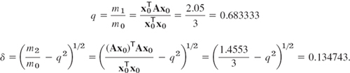
This gives the following values of q, δ, and the error ε = 0.72 − q (calculations with 10D, rounded to 6D):
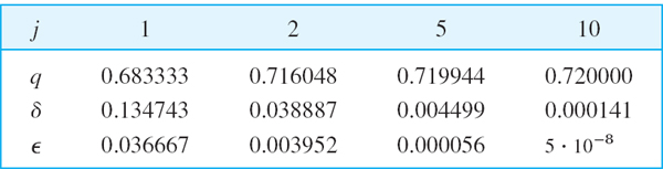
The error bounds are much larger than the actual errors. This is typical, although the bounds cannot be improved; that is, for special symmetric matrices they agree with the errors.
Our present results are somewhat better than those of Collatz's method in Example 4 of Sec. 20.7, at the expense of more operations.
Spectral shift, the transition from A to A − kI, shifts every eigenvalue by −k. Although finding a good k can hardly be made automatic, it may be helped by some other method or small preliminary computational experiments. In Example 1, Gerschgorin's theorem gives −0.02 ![]() λ
λ ![]() 0.82 for the whole spectrum (verify!). Shifting by −0.4 might be too much (then −0.42
0.82 for the whole spectrum (verify!). Shifting by −0.4 might be too much (then −0.42 ![]() λ
λ ![]() 0.42), so let us try −0.2.
0.42), so let us try −0.2.
EXAMPLE 2 Power Method with Spectral Shift
For A − 0.2I with A as in Example 1 we obtain the following substantial improvements (where the index 1 refers to Example 1 and the index 2 to the present example).

1–4 POWER METHOD WITHOUT SCALING
Apply the power method without scaling (3 steps), using x0 = [1, 1]T or [1 1 1]T. Give Rayleigh quotients and error bounds. Show the details of your work.


5–8 POWER METHOD WITH SCALING
Apply the power method (3 steps) with scaling, using x0 = [1 1 1]T or [1 1 1 1]T, as applicable. Give Rayleigh quotients and error bounds. Show the details of your work.
- 5. The matrix in Prob. 3
- 6.

- 7.
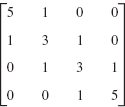
- 8.

- 9. Prove that if x is an eigenvector, then δ = 0 in (2). Give two examples.
- 10. Rayleigh quotient. Why does q generally approximate the eigenvalue of greatest absolute value? When will q be a good approximation?
- 11. Spectral shift, smallest eigenvalue. In Prob. 3 set B = A − 3I (as perhaps suggested by the diagonal entries) and see whether you may get a sequence of q's converging to an eigenvalue of A that is smallest (not largest) in absolute value. Use x0 = [1 1 1]T Do 8 steps. Verify that A has the spectrum {0, 3, 5}.
- 12. CAS EXPERIMENT. Power Method with Scaling. Shifting. (a) Write a program for n × n matrices that prints every step. Apply it to the (nonsymmetric!) matrix (20 steps), starting from [1 1 1]T.
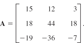
(b) Experiment in (a) with shifting. Which shift do you find optimal?
(c) Write a program as in (a) but for symmetric matrices that prints vectors, scaled vectors, q, and δ. Apply it to the matrix in Prob. 8.
(d). Optimality of δ. Consider
 and take
  . Show that q = 0, δ = 1 for all steps and the eigenvalues are ±1, so that the interval [q − δ, q + δ] cannot be shortened (by omitting ±1) without losing the inclusion property. Experiment with other x0’s.
(e) Find a (nonsymmetric) matrix for which δ in (2) is no longer an error bound.
(f) Experiment systematically with speed of convergence by choosing matrices with the second greatest eigenvalue (i) almost equal to the greatest, (ii) somewhat different, (iii) much different.
20.9 Tridiagonalization and QR-Factorization
We consider the problem of computing all the eigenvalues of a real symmetric matrix A = [ajk], discussing a method widely used in practice. In the first stage we reduce the given matrix stepwise to a tridiagonal matrix, that is, a matrix having all its nonzero entries on the main diagonal and in the positions immediately adjacent to the main diagonal (such as in Fig. 450, Third Step). This reduction was invented by A. S. Householder11 (J. Assn. Comput. Machinery 5 (1958), 335–342). See also Ref. [E29] in App. 1.
This Householder tridiagonalization will simplify the matrix without changing its eigenvalues. The latter will then be determined (approximately) by factoring the tridiagonalized matrix, as discussed later in this section.
Householder's Tridiagonalization Method11
An n × n real symmetric matrix A = [ajk] being given, we reduce it by n − 2 successive similarity transformations (see Sec. 20.6) involving matrices P1, …, Pn−2 to tridiagonal form. These matrices are orthogonal and symmetric. Thus P1−1 = P1T = P1 and similarly for the others. These transformations produce, from the given A0 = A = [ajk], the matrices ![]() in the form
in the form

The transformations (1) create the necessary zeros, in the first step in Row 1 and Column 1, in the second step in Row 2 and Column 2, etc., as Fig. 450 illustrates for a 5 × 5 matrix. B is tridiagonal.
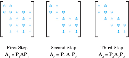
Fig. 450. Householder's method for a 5 × 5 matrix. Positions left blank are zeros created by the method.
How do we determine P1, P2, …, Pn−2? Now, all these Pr are of the form
![]()
where I is the n × n unit matrix and vr = [Ujr] is a unit vector with its first r components 0; thus
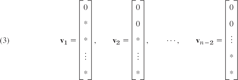
where the asterisks denote the other components (which will be nonzero in general).

where S1 > 0, and sgn a21 = +1 if a21 ![]() 0 and sgn a21 = −1 if a21 < 0. With this we compute P1 by (2) and then A1 by (1). This was the first step.
0 and sgn a21 = −1 if a21 < 0. With this we compute P1 by (2) and then A1 by (1). This was the first step.
Step 2. We compute v2 by (4) with all subscripts increased by 1 and the ajk by ![]() , the entries of A1 just computed. Thus [see also (3)]
, the entries of A1 just computed. Thus [see also (3)]

where
![]()
With this we compute P2 by (2) and then A2 by (1).
Step 3. We compute v3 by (4*) with all subscripts increased by 1 and the ![]() replaced by the entries
replaced by the entries ![]() of A2, and so on.
of A2, and so on.
EXAMPLE 1 Householder Tridiagonalization
Tridiagonalize the real symmetric matrix
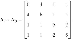
Solution. Step 1. We compute ![]() from (4c). Since a21 = 4 > 0, we have sgn a21 = +1 in (4b) and get from (4) by straightforward computation
from (4c). Since a21 = 4 > 0, we have sgn a21 = +1 in (4b) and get from (4) by straightforward computation
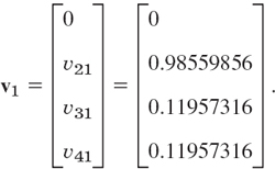
From this and (2),
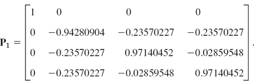
From the first line in (1) we now get

Step 2. From (4*) we compute ![]() and
and

From this and (2),

The second line in (1) now gives
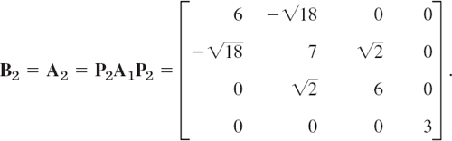
This matrix B is tridiagonal. Since our given matrix has order n = 4, we needed n − 2 = 2 steps to accomplish this reduction, as claimed. (Do you see that we got more zeros than we can expect in general?)
B is similar to A, as we now show in general. This is essential because B thus has the same spectrum as A, by Theorem 2 in Sec. 20.6.
B Similar to A. We assert that B in (1) is similar to A = A0. The matrix Pr is symmetric; indeed,
![]()
Also, Pr is orthogonal because vr is a unit vector, so that ![]() and thus
and thus
Hence ![]() and from (1) we now obtain
and from (1) we now obtain
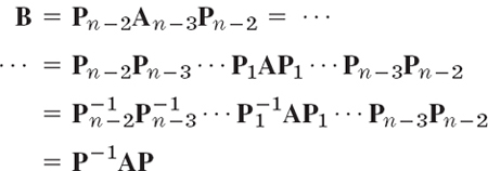
where P = P1P2…Pn−2. This proves our assertion.
QR-Factorization Method
In 1958 H. Rutishauser12 of Switzerland proposed the idea of using the LU-factorization (Sec. 20.2; he called it LR-factorization) in solving eigenvalue problems. An improved version of Rutishauser's method (avoiding breakdown if certain submatrices become singular, etc.; see Ref. [E29]) is the QR-method, independently proposed by the American J. G. F. Francis (Computer J. 4 (1961–62), 265–271, 332–345) and the Russian V. N. Kublanovskaya (Zhurnal Vych. Mat. i Mat. Fiz. 1 (1961), 555–570). The QR-method uses the factorization QR with orthogonal Q and upper triangular R. We discuss the QR-method for a real symmetric matrix. (For extensions to general matrices see Ref. [E29] in App. 1.)
In this method we first transform a given real symmetric n × n matrix A into a tridiagonal matrix B0 = B by Householder's method. This creates many zeros and thus reduces the amount of further work. Then we compute B1, B2, … stepwise according to the following iteration method.
Step 1. Factor B0 = Q0R0 with orthogonal Q0 and upper triangular R0. Then compute B1 = R0Q0.
Step 2. Factor B1 = Q1R1. Then compute B2 = R1Q1.
General Step s + 1.
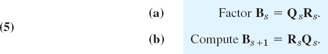
Here Qs is orthogonal and Rs upper triangular. The factorization (5a) will be explained below.
Bs+1 Similar to B. Convergence to a Diagonal Matrix. From (5a) we have ![]() . Substitution into (5b) gives
. Substitution into (5b) gives
![]()
Thus Bs+1 is similar to Bs. Hence Bs+1 is similar to B0 = B for all s. By Theorem 2, Sec. 20.6, this implies that Bs+1 has the same eigenvalues as B.
Also, Bs+1 is symmetric. This follows by induction. Indeed, B0 = B is symmetric. Assuming Bs to be symmetric, that is, BsT = Bs and using ![]() (since Qs is orthogonal), we get from (6) the symmetry,
(since Qs is orthogonal), we get from (6) the symmetry,
![]()
If the eigenvalues of B are different in absolute value, say, |λ1| > |λ2| > … > |λn|, then
![]()
where D is diagonal, with main diagonal entries λ1, λ2, …, λn. (Proof in Ref. [E29] listed in App. 1.)
How to Get the QR-Factorization, say, B = B0 = [bjk] = Q0R0. The tridiagonal matrix B has n − 1 generally nonzero entries below the main diagonal. These are b21, b32, …,bn,n−1. We multiply B from the left by a matrix C2 such that ![]() has
has ![]() . We multiply this by a matrix C3 such that
. We multiply this by a matrix C3 such that ![]() has
has ![]() , etc. After n − 1 such multiplications we are left with an upper triangular matrix R0 namely,
, etc. After n − 1 such multiplications we are left with an upper triangular matrix R0 namely,
![]()
These n × n matrices Cj are very simple. Cj has the 2 × 2 submatrix
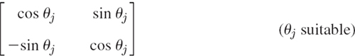
in Rows j − 1 and j and Columns j − 1 and j; everywhere else on the main diagonal the matrix Cj has entries 1; and all its other entries are 0. (This submatrix is the matrix of a plane rotation through the angle θj; see Team Project 30, Sec. 7.2.) For instance, if n = 4, writing cj = cos θj, sj = sin θj, we have

These Cj are orthogonal. Hence their product in (7) is orthogonal, and so is the inverse of this product. We call this inverse Q0. Then from (7),
![]()
where, with ![]() ,
,
![]()
This is our QR-factorization of B0. From it we have by (5b) with s = 0
![]()
We do not need Q0 explicitly, but to get B1 from (10), we first compute ![]() then
then ![]() , etc. Similarly in the further steps that produce B2, B3, ….
, etc. Similarly in the further steps that produce B2, B3, ….
Determination of cos θj and sin θj. We finally show how to find the angles of rotation. cos θ2 and sin θ2 in C2 must be such that ![]() in the product
in the product

Now ![]() is obtained by multiplying the second row of C2 by the first column of B,
is obtained by multiplying the second row of C2 by the first column of B,
![]()
Hence and θ2 = s2/c2 = b21/b11, and
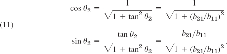
Similarly for θ3, θ4, …. The next example illustrates all this.
EXAMPLE 2 QR-Factorization Method
Compute all the eigenvalues of the matrix
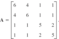
Solution. We first reduce A to tridiagonal form. Applying Householder's method, we obtain (see Example 1)
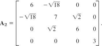
From the characteristic determinant we see that A2, hence A, has the eigenvalue 3. (Can you see this directly from A2?) Hence it suffices to apply the QR-method to the tridiagonal 3 × 3 matrix
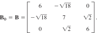
Step 1. We multiply B from the left by

Here ![]() gives (11) cos θ2 = 0.81649658 and sin θ2 = −0.57735027. With these values we compute
gives (11) cos θ2 = 0.81649658 and sin θ2 = −0.57735027. With these values we compute
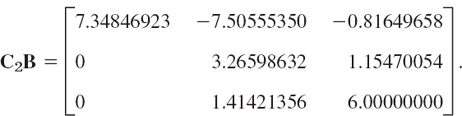
In C3 we get from (−sin θ3) · 3.26598632 + (cos θ3) · 1.41421356 = 0 the values cos θ3 = 0.91766294 and sin θ3 = 0.39735971. This gives

From this we compute

which is symmetric and tridiagonal. The off-diagonal entries in B1 are still large in absolute value. Hence we have to go on.
Step 2. We do the same computations as in the first step, with B0 = B replaced by B1 and C2 and C3 changed accordingly, the new angles being θ2 = −0.196291533 and θ3 = 0.513415589. We obtain
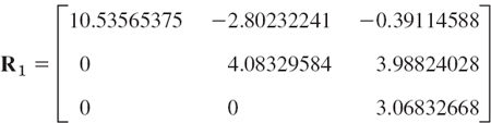
and from this
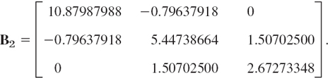
We see that the off-diagonal entries are somewhat smaller in absolute value than those of B1, but still much too large for the diagonal entries to be good approximations of the eigenvalues of B.
Further Steps. We list the main diagonal entries and the absolutely largest off-diagonal entry, which is ![]() in all steps. You may show that the given matrix A has the spectrum 11, 6, 3, 2.
in all steps. You may show that the given matrix A has the spectrum 11, 6, 3, 2.
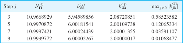
Looking back at our discussion, we recognize that the purpose of applying Householder's tridiagonalization before the QR-factorization method is a substantial reduction of cost in each QR-factorization, in particular if A is large.
Convergence acceleration and thus further reduction of cost can be achieved by a spectral shift, that is, by taking Bs − ksI instead of Bs with a suitable ks. Possible choices of ks are discussed in Ref. [E29], p. 510.
1–5 HOUSEHOLDER TRIDIAGONALIZATION
Tridiagonalize. Show the details.


6–9 QR-FACTORIZATION
Do three QR-steps to find approximations of the eigenvalues of:
- 6. The matrix in the answer to Prob. 1
- 7. The matrix in the answer to Prob. 3
- 8.

- 9.
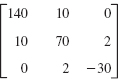
- 10. CAS EXPERIMENT. QR-Method. Try to find out experimentally on what properties of a matrix the speed of decrease of off-diagonal entries in the QR-method depends. For this purpose write a program that first tridiagonalizes and then does QR-steps. Try the program out on the matrices in Probs. 1, 3, and 4. Summarize your findings in a short report.
CHAPTER 20 REVIEW QUESTIONS AND PROBLEMS
- What are the main problem areas in numeric linear algebra?
- When would you apply Gauss elimination and when Gauss–Seidel iteration?
- What is pivoting? Why and how is it done?
- What happens if you apply Gauss elimination to a system that has no solutions?
- What is Cholesky's method? When would you apply it?
- What do you know about the convergence of the Gauss–Seidel iteration?
- What is ill-conditioning? What is the condition number and its significance?
- Explain the idea of least squares approximation.
- What are eigenvalues of a matrix? Why are they important? Give typical examples.
- How did we use similarity transformations of matrices in designing numeric methods?
- What is the power method for eigenvalues? What are its advantages and disadvantages?
- State Gerschgorin's theorem from memory. Give typical applications.
- What is tridiagonalization and QR? When would you apply it?
14–17 GAUSS–SEIDEL ITERATION
Solve
- 14.

- 15.

- 16.
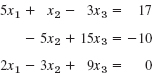
- 17.
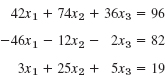
18–20 INVERST MATRIX
Compute the inverse of:
- 18.

- 19.
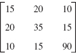
- 20.

21–23 GAUSS–SEIDEL ITERATION
Do 3 steps without scaling, starting from [1 1 1]T.
- 21.

- 22.
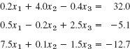
- 23.

24–26 VECTOR NORMS
Compute the ![]() 1-,
1-, ![]() 2-, and
2-, and ![]() ∞-norms of the vectors.
∞-norms of the vectors.
- 24. [0.2 −8.1 0.4 0 0 −1.3 2]T
- 25. [8 −21 13 0]T
- 26. [0 0 0 −1 0]T
27–30 MATRIX NORM
Compute the matrix norm corresponding to the ![]() ∞-vector norm for the coefficient matrix:
∞-vector norm for the coefficient matrix:
- 27. In Prob. 15
- 28. In Prob. 17
- 29. In Prob. 21
- 30. In Prob. 22
31–33 CONDITION NUMBER
Compute the condition number (corresponding to the ![]() ∞-vector norm) of the coefficient matrix:
∞-vector norm) of the coefficient matrix:
- 31. In Prob. 19
- 32. In Prob. 18
- 33. In Prob. 21
34–35 FITTING BY LEAST SQUARES
Fit and graph:
- 34. A straight line to (−1, 0), (0, 2), (1, 2), (2, 3), (3, 3)
- 35. A quadratic parabola to the data in Prob. 34.
Find and graph three circular disks that must contain all the eigenvalues of the matrix:
- 36. In Prob. 18
- 37. In Prob. 19
- 38. In Prob. 20
- 39. Of the coefficients in Prob. 14
- 40. Power method. Do 4 steps with scaling for the matrix in Prob. 19, starting for [1 1 1] and computing the Rayliegh quotients and error bounds.
SUMMARY OF CHAPTER 20 Numeric Linear Algebra
Main tasks are the numeric solution of linear systems (Secs. 20.1–20.4), curve fitting (Sec. 20.5), and eigenvalue problems (Secs. 20.6–20.9).
Linear systems Ax = b with A = [ajk], written out

can be solved by a direct method (one in which the number of numeric operations can be specified in advance, e.g., Gauss's elimination) or by an indirect or iterative method (in which an initial approximation is improved stepwise).
The Gauss elimination (Sec. 20.1) is direct, namely, a systematic elimination process that reduces (1) stepwise to triangular form. In Step 1 we eliminate x1 from equations E2 to En by subtracting (a21/a11) E1 from E2, then (a31/a11) E1 from E3, etc. Equation E1 is called the pivot equation in this step and a11 the pivot. In Step 2 we take the new second equation as pivot equation and eliminate x2, etc. If the triangular form is reached, we get xn from the last equation, then xn−1 from the second last, etc. Partial pivoting (= interchange of equations) is necessary if candidates for pivots are zero, and advisable if they are small in absolute value.
Doolittle's, Crout's, and Cholesky's methods in Sec. 20.2 are variants of the Gauss elimination. They factor A = LU (L lower triangular, U upper triangular) and solve Ax = LUx = b by solving Ly = b for y and then Ux = y for x.
In the Gauss–Seidel iteration (Sec. 20.3) we make a11 = a22 = … = ann = 1 (by division) and write Ax = (I + L + U)x = b; thus x = b − (L + U)x which suggests the iteration formula
![]()
in which we always take the most recent approximate xj’s on the right. If ||C|| < 1, where C = −(I + L)−1U, then this process converges. Here, ||C|| denotes any matrix norm (Sec. 20.3).
If the condition number k(A) = ||A|| ||A−1|| of A is large, then the system Ax = b is ill-conditioned (Sec. 20.4), and a small residual ![]() does not imply that
does not imply that ![]() is close to the exact solution.
is close to the exact solution.
The fitting of a polynomial p(x) = b0 + b1x + … + bmxm through given data (points in the xy-plane) (x1, y1), …, (xn, yn) by the method of least squares is discussed in Sec. 20.5 (and in statistics in Sec. 25.9). If m = n, the least squares polynomial will be the same as an interpolating polynomial (uniqueness).
Eigenvalues λ (values λ for which Ax = λx has a solution x ≠ 0, called an eigenvector) can be characterized by inequalities (Sec. 20.7), e.g. in Gerschgorin's theorem, which gives n circular disks which contain the whole spectrum (all eigenvalues) of A, of centers ajj and radii Σ|ajk| (sum over k from 1 to n, k ≠ j).
Approximations of eigenvalues can be obtained by iteration, starting from an x0 ≠ 0 and computing x1 = Ax0, x2 = Ax1, …,xn = Axn−1. In this power method (Sec. 20.8) the Rayleigh quotient

gives an approximation of an eigenvalue (usually that of the greatest absolute value) and, if A is symmetric, an error bound is
Convergence may be slow but can be improved by a spectral shift.
For determining all the eigenvalues of a symmetric matrix A it is best to first tridiagonalize A and then to apply the QR-method (Sec. 20.9), which is based on a factorization A = QR with orthogonal Q and upper triangular R and uses similarity transformations.
1MYRICK H. DOOLITTLE (1830–1913). American mathematician employed by the U.S. Coast and Geodetic Survey Office. His method appeared in U.S. Coast and Geodetic Survey, 1878, 115–120.
2PRESCOTT DURAND CROUT (1907–1984), American mathematician, professor at MIT, also worked at General Electric.
3ANDRÉ-LOUIS CHOLESKY (1875–1918), French military officer, geodecist, and mathematician. Surveyed Crete and North Africa. Died in World War I. His method was published posthumously in Bulletin Géodésique in 1924 but received little attention until JOHN TODD (1911–2007)—Irish-American mathematician, numerical analysist, and early pioneer of computer methods in numerics, professor at Caltech, and close personal friend and collaborator of ERWIN KREYSZIG, see [E20]—taught Cholesky's method in his analysis course at King's College, London, in the 1940s.
4PHILIPP LUDWIG VON SEIDEL (1821–1896), German mathematician. For Gauss see footnote 5 in Sec. 5.4.
5HENRI LEBESGUE (1875–1941), great French mathematician, creator of a modern theory of measure and integration in his famous doctoral thesis of 1902.
6SEMYON ARANOVICH GERSCHGORIN (1901–1933), Russian mathematician.
7ISSAI SCHUR (1875–1941), German mathematician, also known by his important work in group theory.
8OSKAR PERRON (1880–1975) and GEORG FROBENIUS (1849–1917), German mathematicians, known for their work in potential theory, ODEs (Sec. 5.4), and group theory.
9LOTHAR COLLATZ (1910–1990), German mathematician known for his work in numerics.
10LORD RAYLEIGH (JOHN WILLIAM STRUTT) (1842–1919), great English physicist and mathematician, professor at Cambridge and London, known for his important contributions to various branches of applied mathematics and theoretical physics, in particular, the theory of waves, elasticity, and hydrodynamics. In 1904 he received a Nobel Prize in physics.
11ALSTON SCOTT HOUSEHOLDER (1904–1993), American mathematician, known for his work in numerical analysis and mathematical biology. He was head of the mathematics division at Oakridge National Laboratory and later professor at the University of Tennessee. He was both president of ACM (Association for Computing Machinery) 1954–1956 and SIAM (Society for Industrial and Applied Mathematics) 1963–1964.
12HEINZ RUTISHAUSER (1918–1970). Swiss mathematician, professor at ETH Zurich. Known for his pioneering work in numerics and computer science.