
CHAPTER 13
Complex Numbers and Functions. Complex Differentiation

The transition from “real calculus” to “complex calculus” starts with a discussion of complex numbers and their geometric representation in the complex plane. We then progress to analytic functions in Sec. 13.3. We desire functions to be analytic because these are the “useful functions” in the sense that they are differentiable in some domain and operations of complex analysis can be applied to them. The most important equations are therefore the Cauchy–Riemann equations in Sec. 13.4 because they allow a test of analyticity of such functions. Moreover, we show how the Cauchy–Riemann equations are related to the important Laplace equation.
The remaining sections of the chapter are devoted to elementary complex functions (exponential, trigonometric, hyperbolic, and logarithmic functions). These generalize the familiar real functions of calculus. Detailed knowledge of them is an absolute necessity in practical work, just as that of their real counterparts is in calculus.
Prerequisite: Elementary calculus.
References and Answers to Problems: App. 1 Part D, App. 2.
13.1 Complex Numbers and Their Geometric Representation
The material in this section will most likely be familiar to the student and serve as a review.
Equations without real solutions, such as x2 = −1 or x2 − 10x + 40 = 0, were observed early in history and led to the introduction of complex numbers.1 By definition, a complex number z is an ordered pair (x, y) of real numbers x and y, written
![]()
x is called the real part and y the imaginary part of z, written
![]()
By definition, two complex numbers are equal if and only if their real parts are equal and their imaginary parts are equal.
(0, 1) is called the imaginary unit and is denoted by i,

Addition, Multiplication. Notation z = x + iy
Addition of two complex numbers z1 = (x1, y1) and z2 = (x2,y2) is defined by
![]()
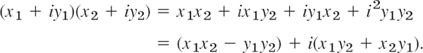
Multiplication is defined by
![]()
These two definitions imply that
![]()
and
![]()
as for real numbers x1, x2. Hence the complex numbers “extend” the real numbers. We can thus write
![]()
because by (1), and the definition of multiplication, we have
![]()
Together we have, by addition, (x, y) = (x, 0) + (0, y) = x + iy.
In practice, complex numbers z = (x, y) are written

or z = x + yi, e.g., 17 + 4i (instead of i4).
Electrical engineers often write j instead of i because they need i for the current. If x = 0, then z = iy and is called pure imaginary. Also, (1) and (3) give

because, by the definition of multiplication, i2 = ii = (0, 1)(0, 1) = (−1, 0) = −1.
For addition the standard notation (4) gives [see (2)]
![]()
For multiplication the standard notation gives the following very simple recipe. Multiply each term by each other term and use i2 = −1 when it occurs [see (3)]:
This agrees with (3). And it shows that x + iy is a more practical notation for complex numbers than (x, y).
If you know vectors, you see that (2) is vector addition, whereas the multiplication (3) has no counterpart in the usual vector algebra.
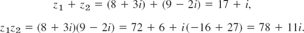
EXAMPLE 1 Real Part, Imaginary Part, Sum and Product of Complex Numbers
Let z1 = 8 + 3i and z2 = 9 − 2i. Then Re z1 = 8, Im z1 = 3, Re z2 = 9, Im z2 = − 2 and
Subtraction, Division
Subtraction and division are defined as the inverse operations of addition and multiplication, respectively. Thus the difference z = z1 − z2 is the complex number z for which z1 = z + z2. Hence by (2),

The quotient z = z1/z2 (z2 ≠ 0) is the complex number z for which z1 = zz2. If we equate the real and the imaginary parts on both sides of this equation, setting z = x + iy, we obtain x1 = x2x − y2y, y1 = y2x + x2y. The solution is

The practical rule used to get this is by multiplying numerator and denominator of z1/z2 by x2 − iy2 and simplifying:

EXAMPLE 2 Difference and Quotient of Complex Numbers
For z1 = 8 + 3i and z2 = 9 − 2i we get z1 − z2 = (8 + 3i) − (9 − 2i) = −1 + 5i and

Check the division by multiplication to get 8 + 3i.
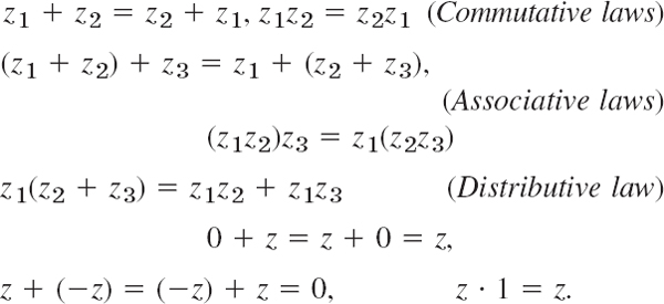
Complex numbers satisfy the same commutative, associative, and distributive laws as real numbers (see the problem set).
Complex Plane
So far we discussed the algebraic manipulation of complex numbers. Consider the geometric representation of complex numbers, which is of great practical importance. We choose two perpendicular coordinate axes, the horizontal x-axis, called the real axis, and the vertical y-axis, called the imaginary axis. On both axes we choose the same unit of length (Fig. 318). This is called a Cartesian coordinate system.


Fig. 319. The number 4 − 3i in the complex plane
We now plot a given complex number z = (x, y) = x + iy as the point P with coordinates x, y. The xy-plane in which the complex numbers are represented in this way is called the complex plane.2 Figure 319 shows an example.
Instead of saying “the point represented by z in the complex plane” we say briefly and simply “the point z in the complex plane.” This will cause no misunderstanding.
Addition and subtraction can now be visualized as illustrated in Figs. 320 and 321.
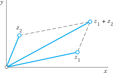
Fig. 320. Addition of complex numbers
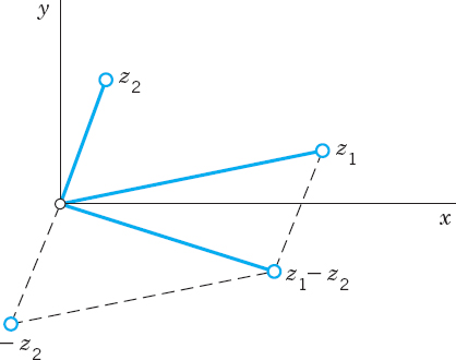
Fig. 321. Subtraction of complex numbers
Complex Conjugate Numbers
The complex conjugate ![]() of a complex number z = x + iy is defined by
of a complex number z = x + iy is defined by

It is obtained geometrically by reflecting the point z in the real axis. Figure 322 shows this for z = 5 + 2i and its conjugate ![]() = 5 − 2i.
= 5 − 2i.
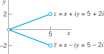
Fig. 322. Complex conjugate numbers
The complex conjugate is important because it permits us to switch from complex to real. Indeed, by multiplication, z![]() = x2 + y2 (verify!). By addition and subtraction, z +
= x2 + y2 (verify!). By addition and subtraction, z + ![]() = 2x, z −
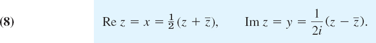
= 2x, z − ![]() = 2iy. We thus obtain for the real part x and the imaginary part y (not iy!) of z =x + iy the important formulas
= 2iy. We thus obtain for the real part x and the imaginary part y (not iy!) of z =x + iy the important formulas
If z is real, z = x, then ![]() = z by the definition of
= z by the definition of ![]() , and conversely. Working with conjugates is easy, since we have
, and conversely. Working with conjugates is easy, since we have

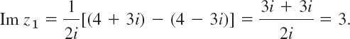
EXAMPLE 3 Illustration of (8) and (9)
Let z1 = 4 + 3i and z2 = 2 + 5i. Then by (8),
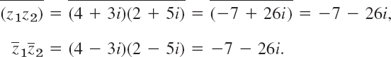
Also, the multiplication formula in (9) is verified by
- Powers of i. Show that i2 = −1, i3 = −i, i4 = 1, i5 = i, … and 1/i = −i, 1/i2 = −1, 1/i3 = i, ….
- Rotation. Multiplication by i is geometrically a counterclockwise rotation through π/2(90°). Verify this by graphing z and iz and the angle of rotation for z = 1 + i, z = −1 + 2i, z = 4 − 3i.
- Division. Verify the calculation in (7). Apply (7) to (26 − 18i)/(6 − 2i).
- Law for conjugates. Verify (9) for z1 = −11 + 10i, z2 = −1 + 4i.
- Pure imaginary number. Show that z = x + iy is pure imaginary if and only if
 = −z.
= −z. - Multiplication. If the product of two complex numbers is zero, show that at least one factor must be zero.
- Laws of addition and multiplication. Derive the following laws for complex numbers from the corresponding laws for real numbers.
8–15 COMPLEX ARITHMETIC
Let z1 = −2 + 11i, z2 = 2 − i. Showing the details of your work, find, in the form x + iy:
- 8.

- 9.
- 10.
- 11. (z1 − z2)2/16, (z1/4 − z2/4)2
- 12. z1/z2, z2/z1
- 13.

- 14.

- 15. 4(z1 + z2)/(z1 − z2)
16–20 Let z = x + iy. Showing details, find, in terms of x and y:
- 16. Im(1/z), Im(1/z2)
- 17. Re z4 − (Rez2)2
- 18. Re [(1 + i)16z2]
- 19. Re(z/), Im (z/)
- 20. Im (1/2)
13.2 Polar Form of Complex Numbers. Powers and Roots
We gain further insight into the arithmetic operations of complex numbers if, in addition to the xy-coordinates in the complex plane, we also employ the usual polar coordinates r, θ defined by

We see that then z = x + iy takes the so-called polar form

r is called the absolute value or modulus of z and is denoted by |z|. Hence
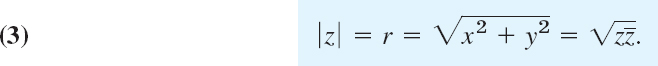
Geometrically, |z| is the distance of the point z from the origin (Fig. 323). Similarly, |z1 − z2| is the distance between z1 and z2 (Fig. 324).
θ is called the argument of z and is denoted by arg z. Thus θ = arg z and (Fig. 323)

Geometrically, θ is the directed angle from the positive x-axis to OP in Fig. 323. Here, as in calculus, all angles are measured in radians and positive in the counterclockwise sense.
For z = 0 this angle θ is undefined. (Why?) For a given z ≠ 0 it is determined only up to integer multiples of 2π since cosine and sine are periodic with period 2π. But one often wants to specify a unique value of arg z of a given z ≠ 0. For this reason one defines the principal value Arg z (with capital A!) of arg z by the double inequality

Then we have Arg z = 0 for positive real z = x, which is practical, and Arg z = π (not −π!) for negative real z, e.g., for z = −4. The principal value (5) will be important in connection with roots, the complex logarithm (Sec. 13.7), and certain integrals. Obviously, for a given z ≠ 0, the other values of arg z are arg z = Arg z ± 2nπ(n = ±1, ±2, …).

Fig. 323. Complex plane, polar form of a complex number

Fig. 324. Distance between two points in the complex plane
EXAMPLE 1 Polar Form of Complex Numbers. Principal Value Arg z
z = 1 + i (Fig. 325) has the polar form. ![]() Hence we obtain
Hence we obtain
![]()
Similarly, ![]() and Arg
and Arg ![]()

Fig. 325. Example 1
CAUTION! In using (4), we must pay attention to the quadrant in which z lies, since tan θ has period π, so that the arguments of z and −z have the same tangent. Example: for θ1 = arg (1 + i) and θ2 = arg (−1 −i) we have tan θ1 = tan θ2 = 1.
Triangle Inequality
Inequalities such as x1 < x2 make sense for real numbers, but not in complex because there is no natural way of ordering complex numbers. However, inequalities between absolute values (which are real!), such as |z1| < |z2 (meaning that z1 is closer to the origin than z2) are of great importance. The daily bread of the complex analyst is the triangle inequality

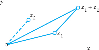
which we shall use quite frequently. This inequality follows by noting that the three points 0, z1 and z1 + z2 are the vertices of a triangle (Fig. 326) with sides |z1|, |z2|, and |z1 + z2|, and one side cannot exceed the sum of the other two sides. A formal proof is left to the reader (Prob. 33). (The triangle degenerates if z1 and z2 lie on the same straight line through the origin.)
By induction we obtain from (6) the generalized triangle inequality

that is, the absolute value of a sum cannot exceed the sum of the absolute values of the terms.
Multiplication and Division in Polar Form
This will give us a “geometrical” understanding of multiplication and division. Let
![]()
Multiplication. By (3) in Sec. 13.1 the product is at first
![]()
The addition rules for the sine and cosine [(6) in App. A3.1] now yield

Taking absolute values on both sides of (7), we see that the absolute value of a product equals the product of the absolute values of the factors,
Taking arguments in (7) shows that the argument of a product equals the sum of the arguments of the factors,

Division. We have z1 = (z1/z2)z2. Hence |z1| = |(z1/z2)z2| = |z1/z2||z2| and by division by |z2|
Similarly, arg z1 = arg [(z1/z2) z2] = arg (z1/z2) + arg z2 and by subtraction of arg z2

Combining (10) and (11) we also have the analog of (7),

To comprehend this formula, note that it is the polar form of a complex number of absolute value r1/r2 and argument θ1 − θ2. But these are the absolute value and argument of z1/z2, as we can see from (10), (11), and the polar forms of z1 and z2.
EXAMPLE 3 Illustration of Formulas (8)–(11)
Let z1 = −2 + 2i and z2 = 3i. Then z1z2 = −6 − 6i, ![]() Hence (make a sketch)
Hence (make a sketch)
![]()
and for the arguments we obtain Arg z1 = 3π/4, Arg z2 = π/2,
![]()
EXAMPLE 4 Integer Powers of z. De Moivre's Formula
From (8) and (9) with z1 = z2 = z we obtain by induction for n = 0, 1, 2, …

Similarly, (12) with z1 = 1 and z2 = zn gives (13) for n = −1, −2, …. For |z| = r = 1, formula (13) becomes De Moivre's formula3

We can use this to express cos nθ and sin nθ in terms of powers of cos θ and sin θ. For instance, for n = 2 we have on the left cos2 θ + 2i cos θ sin θ − sin2 θ. Taking the real and imaginary parts on both sides of (13*) with n = 2 gives the familiar formulas
![]()
This shows that complex methods often simplify the derivation of real formulas. Try n = 3.
Roots
If z = wn (n = 1, 2, …), then to each value of w there corresponds one value of z. We shall immediately see that, conversely, to a given z ≠ 0 there correspond precisely n distinct values of w. Each of these values is called an nth root of z, and we write
Hence this symbol is multivalued, namely, n-valued. The n values of ![]() can be obtained as follows. We write z and w in polar form
can be obtained as follows. We write z and w in polar form
![]()
Then the equation wn = z becomes, by De Moivre's formula (with ø instead of θ),
![]()
The absolute values on both sides must be equal; thus, Rn = r, so that ![]() where
where ![]() is positive real (an absolute value must be nonnegative!) and thus uniquely determined. Equating the arguments nø and θ and recalling that θ is determined only up to integer multiples of 2π, we obtain
is positive real (an absolute value must be nonnegative!) and thus uniquely determined. Equating the arguments nø and θ and recalling that θ is determined only up to integer multiples of 2π, we obtain
![]()
where k is an integer. For k = 0, 1, …, n − 1 we get n distinct values of w. Further integers of k would give values already obtained. For instance, k = n gives 2kπ/n = 2π, hence the w corresponding to k = 0, etc. Consequently, ![]() , for z ≠ 0, has the n distinct values
, for z ≠ 0, has the n distinct values

where k = 0, 1, …, n − 1. These n values lie on a circle of radius ![]() with center at the origin and constitute the vertices of a regular polygon of n sides. The value of
with center at the origin and constitute the vertices of a regular polygon of n sides. The value of ![]() obtained by taking the principal value of arg z and k = 0 in (15) is called the principal value of
obtained by taking the principal value of arg z and k = 0 in (15) is called the principal value of ![]()
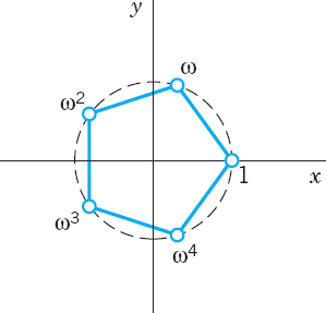
Taking z = 1 in (15), we have |z| = r = 1 and Arg z = 0. Then (15) gives

These n values are called the nth roots of unity. They lie on the circle of radius 1 and center 0, briefly called the unit circle (and used quite frequently!). Figures 327–329 show ![]()


If ω denotes the value corresponding to k = 1 in (16), then the n values of ![]() can be written as
can be written as
![]()
More generally, if w1 is any nth root of an arbitrary complex number z (≠ 0), then the n values of ![]() in (15) are
in (15) are
![]()
because multiplying w1 by ωk corresponds to increasing the argument of w1 by 2kπ/n. Formula (17) motivates the introduction of roots of unity and shows their usefulness.
1–8 POLAR FORM
Represent in polar form and graph in the complex plane as in Fig. 325. Do these problems very carefully because polar forms will be needed frequently. Show the details.
- 1 + i
- −4 + 4i
- 2i, −2i
- −5


9–14 PRINCIPAL ARGUMENT
Determine the principal value of the argument and graph it as in Fig. 325.
- 9. −1 + i
- 10. −5, −5 − i, −5 + i
- 11. 3 ± 4i
- 12. −π − πi
- 13. (1 + i)20
- 14. −1 + 0.1i, −1 − 0.1i
15–18 CONVERSION TO x + iy
Graph in the complex plane and represent in the form x + iy:
- 15.

- 16.

- 17.

- 18.

ROOTS
- 19. CAS PROJECT. Roots of Unity and Their Graphs. Write a program for calculating these roots and for graphing them as points on the unit circle. Apply the program to zn = 1 with n = 2, 3, …, 10. Then extend the program to one for arbitrary roots, using an idea near the end of the text, and apply the program to examples of your choice.
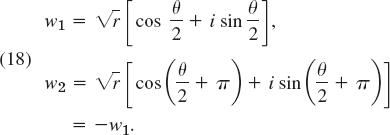
- 20. TEAM PROJECT. Square Root. (a) Show that
 has the values
(b) Obtain from (18) the often more practical formula

where sign y = 1 if y
 0, sign y = −1 if y < 0, and all square roots of positive numbers are taken with positive sign. Hint: Use (10) in App. A3.1 with x = θ/2.
(c) Find the square roots of −14i, −9 − 40i, and
 by both (18) and (19) and comment on the work involved.
 - (d) Do some further examples of your own and apply a method of checking your results.
21–27 ROOTS
Find and graph all roots in the complex plane.
- 21.

- 22.

- 23.

- 24.

- 25.

- 26.

- 27.

28–31 EQUATIONS
Solve and graph the solutions. Show details.
- 28. z2 − (6 − 2i)z + 17 − 6i = 0
- 29. z2 + z + 1 − i = 0
- 30. z4 + 324 = 0. Using the solutions, factor z4 + 324 into quadratic factors with real coefficients.
- 31. z4 − 6iz2 + 16 = 0
32–35 INEQUALITIES AND EQUALITY
- 32. Triangle inequality. Verify (6) for z1 = 3 + i, z2 = −2 + 4i
- 33. Triangle inequality. Prove (6).
- 34. Re and Im. Prove |Re z|
 |z|, |Im z| |z|.
 - 35. Parallelogram equality. Prove and explain the name
![]()
13.3 Derivative. Analytic Function
Just as the study of calculus or real analysis required concepts such as domain, neighborhood, function, limit, continuity, derivative, etc., so does the study of complex analysis. Since the functions live in the complex plane, the concepts are slightly more difficult or different from those in real analysis. This section can be seen as a reference section where many of the concepts needed for the rest of Part D are introduced.
Circles and Disks. Half-Planes
The unit circle |z| = 1 (Fig. 330) has already occurred in Sec. 13.2. Figure 331 shows a general circle of radius ρ and center a. Its equation is
![]()

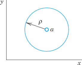
Fig. 331. Circle in the complex plane

Fig. 332. Annulus in the complex plane
because it is the set of all z whose distance |z − a| from the center a equals ρ. Accordingly, its interior (“open circular disk”) is given by |z − a| < ρ, its interior plus the circle itself (“closed circular disk”) by |z − a| ![]() ρ, and its exterior by |z − a| > ρ. As an example, sketch this for a = 1 + i and ρ = 2, to make sure that you understand these inequalities.
ρ, and its exterior by |z − a| > ρ. As an example, sketch this for a = 1 + i and ρ = 2, to make sure that you understand these inequalities.
An open circular disk |z − a| < ρ is also called a neighborhood of a or, more precisely, a ρ-neighborhood of a. And a has infinitely many of them, one for each value of ρ(>0), and a is a point of each of them, by definition!
In modern literature any set containing a ρ-neighborhood of a is also called a neighborhood of a.
Figure 332 shows an open annulus (circular ring) ρ1 < |z − a| <ρ2, which we shall need later. This is the set of all z whose distance |z − a| from a is greater than ρ1 but less than ρ2. Similarly, the closed annulus ρ1 ![]() |z − a|
|z − a| ![]() ρ2 includes the two circles.
ρ2 includes the two circles.
Half-Planes. By the (open) upper half-plane we mean the set of all points z = x + iy such that y > 0. Similarly, the condition y < 0 defines the lower half-plane, x > 0 the right half-plane, and x < 0 the left half-plane.
For Reference: Concepts on Sets in the Complex Plane
To our discussion of special sets let us add some general concepts related to sets that we shall need throughout Chaps. 13–18; keep in mind that you can find them here.
By a point set in the complex plane we mean any sort of collection of finitely many or infinitely many points. Examples are the solutions of a quadratic equation, the points of a line, the points in the interior of a circle as well as the sets discussed just before.
A set S is called open if every point of S has a neighborhood consisting entirely of points that belong to S. For example, the points in the interior of a circle or a square form an open set, and so do the points of the right half-plane Re z = x > 0.
A set S is called connected if any two of its points can be joined by a chain of finitely many straight-line segments all of whose points belong to S. An open and connected set is called a domain. Thus an open disk and an open annulus are domains. An open square with a diagonal removed is not a domain since this set is not connected. (Why?)
The complement of a set S in the complex plane is the set of all points of the complex plane that do not belong to S. A set S is called closed if its complement is open. For example, the points on and inside the unit circle form a closed set (“closed unit disk”) since its complement |z| > 1 is open.
A boundary point of a set S is a point every neighborhood of which contains both points that belong to S and points that do not belong to S. For example, the boundary points of an annulus are the points on the two bounding circles. Clearly, if a set S is open, then no boundary point belongs to S; if S is closed, then every boundary point belongs to S. The set of all boundary points of a set S is called the boundary of S.
A region is a set consisting of a domain plus, perhaps, some or all of its boundary points. WARNING! “Domain” is the modern term for an open connected set. Nevertheless, some authors still call a domain a “region” and others make no distinction between the two terms.
Complex Function
Complex analysis is concerned with complex functions that are differentiable in some domain. Hence we should first say what we mean by a complex function and then define the concepts of limit and derivative in complex. This discussion will be similar to that in calculus. Nevertheless it needs great attention because it will show interesting basic differences between real and complex calculus.
Recall from calculus that a real function f defined on a set S of real numbers (usually an interval) is a rule that assigns to every x in S a real number f(x), called the value of f at x. Now in complex, S is a set of complex numbers. And a function f defined on S is a rule that assigns to every z in S a complex number w, called the value of f at z. We write
![]()
Here z varies in S and is called a complex variable. The set S is called the domain of definition of f or, briefly, the domain of f. (In most cases S will be open and connected, thus a domain as defined just before.)
Example: w = f(z) = z2 + 3z is a complex function defined for all z; that is, its domain S is the whole complex plane.
The set of all values of a function f is called the range of f.
w is complex, and we write w = u + iv, where u and v are the real and imaginary parts, respectively. Now w depends on z = x + iy. Hence u becomes a real function of x and y, and so does v. We may thus write
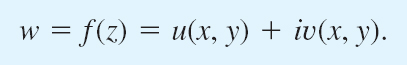
This shows that a complex function f(z) is equivalent to a pair of real functions u(x, y) and v(x, y), each depending on the two real variables x and y.
EXAMPLE 1 Function of a Complex Variable
Let w = f(z) = z2 + 3z. Find u and v and calculate the value of f at z = 1 + 3i.
Solution. u = Re f(z) = x2 − y2 + 3x and v = 2xy + 3y. Also,
![]()
This shows that u(1, 3) = −5 and v(1, 3) = 15. Check this by using the expressions for u and v.
EXAMPLE 2 Function of a Complex Variable
Let w = f(z) = 2iz + 6![]() . Find u and v and the value of f at
. Find u and v and the value of f at ![]()
Solution. f(z) = 2i(x + iy) + 6(x − iy) gives u(x, y) = 6x − 2y and v(x, y) = 2x − 6y. Also,
![]()
Check this as in Example 1.
Remarks on Notation and Terminology
1. Strictly speaking, f(z) denotes the value of f at z, but it is a convenient abuse of language to talk about the function f(z) (instead of the function f), thereby exhibiting the notation for the independent variable.
2. We assume all functions to be single-valued relations, as usual: to each z in S there corresponds but one value w = f(z) (but, of course, several z may give the same value w = f(z), just as in calculus). Accordingly, we shall not use the term “multivalued function” (used in some books on complex analysis) for a multivalued relation, in which to a z there corresponds more than one w.
Limit, Continuity
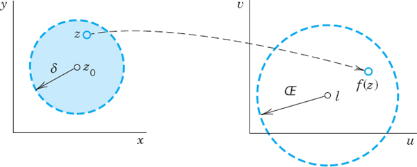
A function f(z) is said to have the limit l as z approaches a point z0, written
![]()
if f is defined in a neighborhood of z0 (except perhaps at z0 itself) and if the values of f are “close” to l for all z “close” to z0; in precise terms, if for every positive real ![]() we can find a positive real δ such that for all z ≠ z0 in the disk |z − z0| < δ (Fig. 333) we have
we can find a positive real δ such that for all z ≠ z0 in the disk |z − z0| < δ (Fig. 333) we have
![]()
geometrically, if for every z ≠ z0 in that δ-disk the value of f lies in the disk (2).
Formally, this definition is similar to that in calculus, but there is a big difference. Whereas in the real case, x can approach an x0 only along the real line, here, by definition, z may approach z0 from any direction in the complex plane. This will be quite essential in what follows.
If a limit exists, it is unique. (See Team Project 24.)
A function f(z) is said to be continuous at z = z0 if f(z0) is defined and
![]()
Note that by definition of a limit this implies that f(z) is defined in some neighborhood of z0.
f(z) is said to be continuous in a domain if it is continuous at each point of this domain.
Derivative
The derivative of a complex function f at a point z0 is written f′(z0) and is defined by
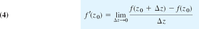
provided this limit exists. Then f is said to be differentiable at z0. If we write Δz = z − z0, we have z = z0 + Δz and (4) takes the form

Now comes an important point. Remember that, by the definition of limit, f(z) is defined in a neighborhood of z0 and z in (4′) may approach z0 from any direction in the complex plane. Hence differentiability at z0 means that, along whatever path z approaches z0, the quotient in (4′) always approaches a certain value and all these values are equal. This is important and should be kept in mind.
EXAMPLE 3 Differentiability. Derivative
The function f(z) = z2 is differentiable for all z and has the derivative f′(z) = 2z because
![]()
The differentiation rules are the same as in real calculus, since their proofs are literally the same. Thus for any differentiable functions f and g and constant c we have

as well as the chain rule and the power rule (zn)′ = nzn−1(n integer).
Also, if f(z) is differentiable at z0, it is continuous at z0. (See Team Project 24.)
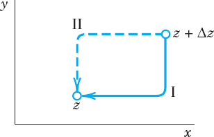
It may come as a surprise that there are many complex functions that do not have a derivative at any point. For instance, f(z) = ![]() = x − iy is such a function. To see this, we write Δz = Δx + iΔy and obtain
= x − iy is such a function. To see this, we write Δz = Δx + iΔy and obtain

If Δy = 0, this is +1. If Δx = 0, this is −1. Thus (5) approaches +1 along path I in Fig. 334 but −1 along path II. Hence, by definition, the limit of (5) as Δz→0 does not exist at any z.
Surprising as Example 4 may be, it merely illustrates that differentiability of a complex function is a rather severe requirement.
The idea of proof (approach of z from different directions) is basic and will be used again as the crucial argument in the next section.
Analytic Functions
Complex analysis is concerned with the theory and application of “analytic functions,” that is, functions that are differentiable in some domain, so that we can do “calculus in complex.” The definition is as follows.
A function f(z) is said to be analytic in a domain D if f(z) is defined and differentiable at all points of D. The function f(z) is said to be analytic at a point z = z0 in D if f(z) is analytic in a neighborhood of z0.
Also, by an analytic function we mean a function that is analytic in some domain.
Hence analyticity of f(z) at z0 means that f(z) has a derivative at every point in some neighborhood of z0 (including z0 itself since, by definition, z0 is a point of all its neighborhoods). This concept is motivated by the fact that it is of no practical interest if a function is differentiable merely at a single point z0 but not throughout some neighborhood of z0. Team Project 24 gives an example.
A more modern term for analytic in D is holomorphic in D.
EXAMPLE 5 Polynomials, Rational Functions
The nonnegative integer powers 1, z, z2, … are analytic in the entire complex plane, and so are polynomials, that is, functions of the form
![]()
where c0, …,cn are complex constants.
The quotient of two polynomials g(z) and h(z),
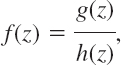
is called a rational function. This f is analytic except at the points where h(z) = 0; here we assume that common factors of g and h have been canceled.
Many further analytic functions will be considered in the next sections and chapters.
The concepts discussed in this section extend familiar concepts of calculus. Most important is the concept of an analytic function, the exclusive concern of complex analysis. Although many simple functions are not analytic, the large variety of remaining functions will yield a most beautiful branch of mathematics that is very useful in engineering and physics.
1–8 REGIONS OF PRACTICAL INTEREST
Determine and sketch or graph the sets in the complex plane given by

- 0 < |z| < 1
- π < |z − 4 + 2i| < 3π
- −π < Im z < π

- Re (1/z) < 1
- Re z −1
- |z + i| |z − i|
- WRITING PROJECT. Sets in the Complex Plane. Write a report by formulating the corresponding portions of the text in your own words and illustrating them with examples of your own.
COMPLEX FUNCTIONS AND THEIR DERIVATIVES
10–12 Function Values. Find Re f, and Im f and their values at the given point z.
- 10. f(z) = 5z2 − 12z + 3 + 2i at 4 − 3i
- 11. f(z) = 1/(1 − z) at 1 − i
- 12. f(z) = (z − 2)/(z + 2) at 8i
- 13. CAS PROJECT. Graphing Functions. Find and graph Re f, Im f, and |f| as surfaces over the z-plane. Also graph the two families of curves and Re f(z) = const and Im f(z) = const in the same figure, and the curves |f(z)| = const in another figure, where (a)f(z) = z2, (b) f(z) = 1/z, (c) f(z) = z4.
14–17 Continuity. Find out, and give reason, whether f(z) is continuous at z = 0 if f(0) = 0 and for z ≠ 0 the function f is equal to:
- 14. (Re z2)/|z|
- 15. |z|2 Im (1/z)
- 16. (Im z2)/|z|2
- 17. (Re z)/(1 − |z|)
18–23 Differentiation. Find the value of the derivative of
- 18. (z − i)/(z + i) ati
- 19. (z − 4i)8 at = 3 + 4i
- 20. (1.5z + 2i)/(3iz − 4) at any z. Explain the result.
- 21. i(1 − z)n at 0
- 22. (iz3 + 3z2)3 at 2i
- 23. z3/(z + i)3 at i
- 24. TEAM PROJECT. Limit, Continuity, Derivative
(a) Limit. Prove that (1) is equivalent to the pair of relations

(b) Limit. If
 exists, show that this limit is unique.
(c) Continuity. If z1, z2, … are complex numbers for which
 and if f(z) is continuous at z = a, show that
(d) Continuity. If f(z) is differentiable at z0, show that f(z) is continuous at z0.
(e) Differentiability. Show that f(z) = Re z = x is not differentiable at any z. Can you find other such functions?
(f) Differentiability. Show that f(z) = |z|2 is differentiable only at z = 0; hence it is nowhere analytic.
- 25. WRITING PROJECT. Comparison with Calculus. Summarize the second part of this section beginning with Complex Function, and indicate what is conceptually analogous to calculus and what is not.
13.4 Cauchy–Riemann Equations. Laplace's Equation
As we saw in the last section, to do complex analysis (i.e., “calculus in the complex”) on any complex function, we require that function to be analytic on some domain that is differentiable in that domain.
The Cauchy–Riemann equations are the most important equations in this chapter and one of the pillars on which complex analysis rests. They provide a criterion (a test) for the analyticity of a complex function
![]()
Roughly, f is analytic in a domain D if and only if the first partial derivatives of u and v satisfy the two Cauchy–Riemann equations4

everywhere in D; here ux = ∂u/∂y and uy = ∂u/∂y (and similarly for v) are the usual notations for partial derivatives. The precise formulation of this statement is given in Theorems 1 and 2.
Example: f(z) = z2 = x2 − y2 + 2ixy is analytic for all z (see Example 3 in Sec. 13.3), and u = x2 − y2 and v = 2xy satisfy (1), namely, ux = 2x = vy as well as uy = −2y = −vx. More examples will follow.
THEOREM 1 Cauchy–Riemann Equations
Let f(z) = u(x, y) + iv(x, y) be defined and continuous in some neighborhood of a point z = x + iy and differentiable at z itself. Then, at that point, the first-order partial derivatives of u and v exist and satisfy the Cauchy–Riemann equations (1).
Hence, if f(z) is analytic in a domain D, those partial derivatives exist and satisfy (1) at all points of D.
By assumption, the derivative f′(z) at z exists. It is given by

The idea of the proof is very simple. By the definition of a limit in complex (Sec. 13.3), we can let Δz approach zero along any path in a neighborhood of z. Thus we may choose the two paths I and II in Fig. 335 and equate the results. By comparing the real parts we shall obtain the first Cauchy–Riemann equation and by comparing the imaginary parts the second. The technical details are as follows.
We write Δz = Δx + i Δy. Then z + Δz = x + Δx + i(y + Δy), and in terms of u and v the derivative in (2) becomes

We first choose path I in Fig. 335. Thus we let Δy → 0 first and then Δx → 0. After Δy is zero, Δz = Δx. Then (3) becomes, if we first write the two u-terms and then the two v-terms,
![]()

Since f′(z) exists, the two real limits on the right exist. By definition, they are the partial derivatives of u and v with respect to x. Hence the derivative f′(z) of f(z) can be written

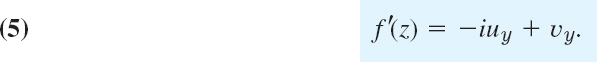
Similarly, if we choose path II in Fig. 335, we let Δx → 0 first and then Δy → 0. After Δx is zero, Δz = i Δy, so that from (3) we now obtain

Since f′(z) exists, the limits on the right exist and give the partial derivatives of u and v with respect to y; noting that 1/i = −i, we thus obtain
The existence of the derivative f′(z) thus implies the existence of the four partial derivatives in (4) and (5). By equating the real parts ux and vy in (4) and (5) we obtain the first Cauchy–Riemann equation (1). Equating the imaginary parts gives the other. This proves the first statement of the theorem and implies the second because of the definition of analyticity.
Formulas (4) and (5) are also quite practical for calculating derivatives f′(z) as we shall see.
EXAMPLE 1 Cauchy–Riemann Equations
f(z) = z2 is analytic for all z. It follows that the Cauchy–Riemann equations must be satisfied (as we have verified above).
For f(z) = ![]() = x − iy we have u = x, v = −y and see that the second Cauchy–Riemann equation is satisfied, uy = −vx = 0, but the first is not: ux = 1 ≠ vy = −1. We conclude that f(z) =
= x − iy we have u = x, v = −y and see that the second Cauchy–Riemann equation is satisfied, uy = −vx = 0, but the first is not: ux = 1 ≠ vy = −1. We conclude that f(z) = ![]() is not analytic, confirming Example 4 of Sec. 13.3. Note the savings in calculation!
is not analytic, confirming Example 4 of Sec. 13.3. Note the savings in calculation!
The Cauchy–Riemann equations are fundamental because they are not only necessary but also sufficient for a function to be analytic. More precisely, the following theorem holds.
THEOREM 2 Cauchy–Riemann Equations
If two real-valued continuous functions u(x, y) and v(x, y) of two real variables x and y have continuous first partial derivatives that satisfy the Cauchy–Riemann equations in some domain D, then the complex function f(z) = u(x, y) + iv(x, y) is analytic in D.
The proof is more involved than that of Theorem 1 and we leave it optional (see App. 4).
Theorems 1 and 2 are of great practical importance, since, by using the Cauchy–Riemann equations, we can now easily find out whether or not a given complex function is analytic.
EXAMPLE 2 Cauchy–Riemann Equations. Exponential Function
Is f(z) = u(x, y) + iv(x, y) = ex(cos y + i sin y) analytic?
Solution. We have u = ex cos y, v = ex sin y and by differentiation
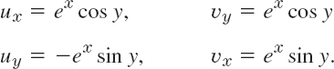
We see that the Cauchy–Riemann equations are satisfied and conclude that f(z) is analytic for all z. (f(z) will be the complex analog of ex known from calculus.)
EXAMPLE 3 An Analytic Function of Constant Absolute Value Is Constant
The Cauchy–Riemann equations also help in deriving general properties of analytic functions.
For instance, show that if f(z) is analytic in a domain D and |f(z)| = k = const in D, then f(z) = const in D. (We shall make crucial use of this in Sec. 18.6 in the proof of Theorem 3.)
Solution. By assumption, |f|2 = |u + iv|2 = u2 + v2 = k2. By differentiation,
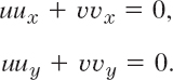
Now use vx = −uy in the first equation and vy = ux in the second, to get
To get rid of uy, multiply (6a) by u and (6b) by v and add. Similarly, to eliminate ux, multiply (6a) by −v and (6b) by u and add. This yields

If k2 = u2 + v2 = 0, then u = v = 0; hence f = 0. If k2 = u2 + v2 ≠ 0, then ux = uy = 0. Hence, by the Cauchy–Riemann equations, also ux = vy = 0. Together this implies u = const and v = const; hence f = const.
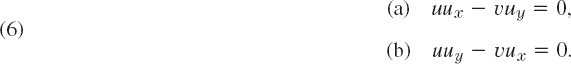
We mention that, if we use the polar form z = r(cos θ + i sin θ) and set f(z) = u(r, θ) + iv(r, θ), then the Cauchy–Riemann equations are (Prob. 1)
Laplace's Equation. Harmonic Functions
The great importance of complex analysis in engineering mathematics results mainly from the fact that both the real part and the imaginary part of an analytic function satisfy Laplace's equation, the most important PDE of physics. It occurs in gravitation, electrostatics, fluid flow, heat conduction, and other applications (see Chaps. 12 and 18).
If f(z) = u(x, y) + iv(x, y) is analytic in a domain D, then both u and v satisfy Laplace's equation
![]()
(∇2 read “nabla squared”) and
![]()
in D and have continuous second partial derivatives in D.
PROOF
Differentiating ux = vy with respect to x and uy = −vx with respect to y, we have
![]()
Now the derivative of an analytic function is itself analytic, as we shall prove later (in Sec. 14.4). This implies that u and v have continuous partial derivatives of all orders; in particular, the mixed second derivatives are equal: vyx = vxy. By adding (10) we thus obtain (8). Similarly, (9) is obtained by differentiating ux = vy with respect to y and uy = −vx with respect to x and subtracting, using uxy = uyx.
Solutions of Laplace's equation having continuous second-order partial derivatives are called harmonic functions and their theory is called potential theory (see also Sec. 12.11). Hence the real and imaginary parts of an analytic function are harmonic functions.
If two harmonic functions u and v satisfy the Cauchy–Riemann equations in a domain D, they are the real and imaginary parts of an analytic function f in D. Then v is said to be a harmonic conjugate function of u in D. (Of course, this has absolutely nothing to do with the use of “conjugate” for ![]() .)
.)
EXAMPLE 4 How to Find a Harmonic Conjugate Function by the Cauchy–Riemann Equations
Verify that u = x2 − y2 − y is harmonic in the whole complex plane and find a harmonic conjugate function v of u.
Solution. ![]() by direct calculation. Now ux = 2x and uy = −2y − 1. Hence because of the Cauchy–Riemann equations a conjugate v of u must satisfy
by direct calculation. Now ux = 2x and uy = −2y − 1. Hence because of the Cauchy–Riemann equations a conjugate v of u must satisfy
![]()
Integrating the first equation with respect to y and differentiating the result with respect to x, we obtain

A comparison with the second equation shows that dh/dx = 1. This gives h(x) = x + c. Hence v = 2xy + x + c (c any real constant) is the most general harmonic conjugate of the given u. The corresponding analytic function is
![]()
Example 4 illustrates that a conjugate of a given harmonic function is uniquely determined up to an arbitrary real additive constant.
The Cauchy–Riemann equations are the most important equations in this chapter. Their relation to Laplace's equation opens a wide range of engineering and physical applications, as shown in Chap. 18.
- Cauchy–Riemann equations in polar form. Derive (7) from (1).
2–11 CAUCHY–RIEMANN EQUATIONS
Are the following functions analytic? Use (1) or (7).
- 2.

- 3. f(z) = e−2x (cos 2y − i sin 2y)
- 4. f(z) = ex (cos y − i sin y)
- 5. f(z) = Re(z2) − i Im (z2)
- 6. f(z) = 1/(z − z5)
- 7. f(z) = i/z8
- 8. f(z) = Arg 2πz
- 9. f(z) = 3π2/(z3 + 4π2z)
- 10. f(z) = ln |z| + i Arg z
- 11. f(z) = cos x cosh y − i sin x sinh y
12–19 HARMONIC FUNCTIONS
Are the following functions harmonic? If your answer is yes, find a corresponding analytic function f(z) = u(x, y) + iv(x, y).
- 12. u = x2 + y2
- 13. u = xy
- 14. v = xy
- 15. u = x/(x2 + y2)
- 16. u = sin x cosh y
- 17. v = (2x + 1)y
- 18. u = x3 − 3xy2
- 19. v = ex sin 2y
- 20. Laplace's equation. Give the details of the derivative of (9).
21–24 Determine a and b so that the given function is harmonic and find a harmonic conjugate.
- 21. u = eπx cos av
- 22. u = cos ax cosh 2y
- 23. u = ax3 + bxy
- 24. u = cosh ax cos y
- 25. CAS PROJECT. Equipotential Lines. Write a program for graphing equipotential lines u = const of a harmonic function u and of its conjugate v on the same axes. Apply the program to (a) u = x2 − y2, v = 2xy, (b) u = x3 − 3xy2, v = 3x2y − y3.
- 26. Apply the program in Prob. 25 to u = ex cos y, v = ex sin y and to an example of your own.
- 27. Harmonic conjugate. Show that if u is harmonic and v is a harmonic conjugate of u, then u is a harmonic conjugate of −v.
- 28. Illustrate Prob. 27 by an example.
- 29. Two further formulas for the derivative. Formulas (4), (5), and (11) (below) are needed from time to time. Derive

- 30. TEAM PROJECT. Conditions for f(z) = const. Let f(z) be analytic. Prove that each of the following conditions is sufficient for f(z) = const.
- Re f(z) = const
- Im f(z) = const
- f′(z) = 0
- |f(z)| = const (see Example 3)
13.5 Exponential Function
In the remaining sections of this chapter we discuss the basic elementary complex functions, the exponential function, trigonometric functions, logarithm, and so on. They will be counterparts to the familiar functions of calculus, to which they reduce when z = x is real. They are indispensable throughout applications, and some of them have interesting properties not shared by their real counterparts.
We begin with one of the most important analytic functions, the complex exponential function
![]()
The definition of ex in terms of the real functions ex, cos y, and sin y is

This definition is motivated by the fact the ez extends the real exponential function ex of calculus in a natural fashion. Namely:
(A) ez = ex for real z = x because cos y = 1 and sin y = 0 when y = 0.
(B) ez is analytic for all z. (Proved in Example 2 of Sec. 13.4.)
(C) The derivative of ez is ez, that is,
![]()
This follows from (4) in Sec. 13.4,
![]()
REMARK. This definition provides for a relatively simple discussion. We could define ez by the familiar series 1 + x + x2/2! + x3/3! + … with x replaced by z, but we would then have to discuss complex series at this very early stage. (We will show the connection in Sec. 15.4.)
Further Properties. A function f(z) that is analytic for all z is called an entire function. Thus, ez is entire. Just as in calculus the functional relation
![]()
holds for any and z1 = x1 + iy1 and z2 = x2 + iy2 Indeed, by (1),
![]()
Since ex1ex2 = ex1+x2 for these real functions, by an application of the addition formulas for the cosine and sine functions (similar to that in Sec. 13.2) we see that
![]()
as asserted. An interesting special case of (3) is z1 = x, z2 = iy; then
![]()
Furthermore, for z = iy we have from (1) the so-called Euler formula
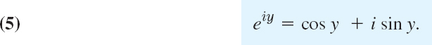
Hence the polar form of a complex number, z = r(cos θ + i sin θ), may now be written
From (5) we obtain

as well as the important formulas (verify!)
![]()
Another consequence of (5) is
![]()
That is, for pure imaginary exponents, the exponential function has absolute value 1, a result you should remember. From (9) and (1),
![]()
since |ez| = ex shows that (1) is actually ez in polar form.
From |ez| = ex ≠ 0 in (10) we see that

So here we have an entire function that never vanishes, in contrast to (nonconstant) polynomials, which are also entire (Example 5 in Sec. 13.3) but always have a zero, as is proved in algebra.
Periodicity of ex with period 2πi,
![]()
is a basic property that follows from (1) and the periodicity of cos y and sin y. Hence all the values that w = ez can assume are already assumed in the horizontal strip of width 2π

This infinite strip is called a fundamental region of ez.
EXAMPLE 1 Function Values. Solution of Equations
Computation of values from (1) provides no problem. For instance,

To illustrate (3), take the product of
![]()
and verify that it equals. e2e4(cos2 1 + sin2 1) = e6 = e(2+i)+(4−i)
To solve the equation ez = 3 + 4i, note first that |ez| = ex = 5, x = ln 5 = 1.609 is the real part of all solutions. Now, since ex = 5,
![]()
Ans. z = 1.609 + 0.927i ± 2nπi (n = 0, 1, 2, …). These are infinitely many solutions (due to the periodicity of ez). They lie on the vertical line x = 1.609 at a distance 2π from their neighbors.
To summarize: many properties of ez = exp z parallel those of ex; an exception is the periodicity of ez with 2πi, which suggested the concept of a fundamental region. Keep in mind that ez is an entire function. (Do you still remember what that means?)

Fig. 336. Fundamental region of the exponential function ez in the z-plane
- ez is entire. Prove this.
2–7 Function Values. Find ez in the form u + iv and |ez| if z equals
- 2. 3 + 4i
- 3. 2πi(1 + i)
- 4. 0.6 − 1.8i
- 5. 2 + 3πi
- 6. 11πi/2
- 7.

8–13 Polar Form. Write in exponential form (6):
- 8.

- 9. 4 + 3i
- 10.

- 11. −6.3
- 12. 1/(1 − z)
- 13. 1 + i
14–17 Real and Imaginary Parts. Find Re and Im of
- 14. e−πz
- 15. exp (z2)
- 16. e1/z
- 17. exp (z3)
- 18. TEAM PROJECT. Further Properties of the Exponential Function. (a) Analyticity. Show that ez is entire. What about
 ? (Use the Cauchy–Riemann equations.)
(b) Special values. Find all z such that (i) ez is real, (ii) |e−z| < 1, (iii)

(c) Harmonic function. Show that u = exy cos (x2/2 − y2/2) is harmonic and find a conjugate.
(d) Uniqueness. It is interesting that f(z) = ez is uniquely determined by the two properties f(x + i0) = ex and f′(z) = f(z), where f is assumed to be entire. Prove this using the Cauchy–Riemann equations.
19–22 Equations. Find all solutions and graph some of them in the complex plane.
- 19. ex = 1
- 20. ex = 4 + 3i
- 21. ex = 0
- 22. ez = −2
13.6 Trigonometric and Hyperbolic Functions. Euler's Formula
Just as we extended the real ex to the complex ez in Sec. 13.5, we now want to extend the familiar real trigonometric functions to complex trigonometric functions. We can do this by the use of the Euler formulas (Sec. 13.5)
![]()
By addition and subtraction we obtain for the real cosine and sine

This suggests the following definitions for complex values z = x + iy:

It is quite remarkable that here in complex, functions come together that are unrelated in real. This is not an isolated incident but is typical of the general situation and shows the advantage of working in complex.
Furthermore, as in calculus we define

and

Since ez is entire, cos z and sin z are entire functions. tan z and sec z are not entire; they are analytic except at the points where cos z is zero; and cot z and csc z are analytic except where sin z is zero. Formulas for the derivatives follow readily from (ez)′ = ez and (1)–(3); as in calculus,
![]()
etc. Equation (1) also shows that Euler's formula is valid in complex:

The real and imaginary parts of cos z and sin z are needed in computing values, and they also help in displaying properties of our functions. We illustrate this with a typical example.
EXAMPLE 1 Real and Imaginary Parts. Absolute Value. Periodicity
Show that

and
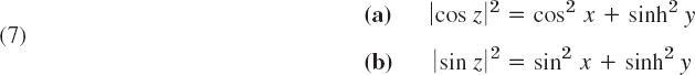
and give some applications of these formulas.
Solution. From (1),

This yields (6a) since, as is known from calculus,
![]()
(6b) is obtained similarly. From (6a) and cosh2y = 1 + sinh2y we obtain
![]()
Since sin2x + cos2x = 1, this gives (7a), and (7b) is obtained similarly.
For instance, cos (2 + 3i) = cos 2 cosh 3 −i sin 2 sinh 3 = −4.190 − 9.109i.
From (6) we see that sin z and cos z are periodic with period 2π, just as in real. Periodicity of tan z and cot z with period π now follows.
Formula (7) points to an essential difference between the real and the complex cosine and sine; whereas |cos x| ![]() 1 and |sin x|
1 and |sin x| ![]() 1, the complex cosine and sine functions are no longer bounded but approach infinity in absolute value as y → ∞, since then sinh y → ∞ in (7).
1, the complex cosine and sine functions are no longer bounded but approach infinity in absolute value as y → ∞, since then sinh y → ∞ in (7).
EXAMPLE 2 Solutions of Equations. Zeros of cos z and sin z
Solve (a) cos z = 5 (which has no real solution!), (b) cos z = 0, (c) sin z = 0.
Solution. (a) e2iz − 10eiz + 1 = 0 from (1) by multiplication by eiz. This is a quadratic equation in eiz, with solutions (rounded off to 3 decimals)
![]()
Thus e−y = 9.899 or 0.101, eix = 1, y = ±2.292, x = 2nπ. Ans. z = ±2nπ ± 2.292i (n = 0, 1, 2, …).
Can you obtain this from (6a)?
General formulas for the real trigonometric functions continue to hold for complex values. This follows immediately from the definitions. We mention in particular the addition rules

and the formula
![]()
Some further useful formulas are included in the problem set.
Hyperbolic Functions
The complex hyperbolic cosine and sine are defined by the formulas

This is suggested by the familiar definitions for a real variable [see (8)]. These functions are entire, with derivatives
![]()
as in calculus. The other hyperbolic functions are defined by

Complex Trigonometric and Hyperbolic Functions Are Related. If in (11), we replace z by iz and then use (1), we obtain

Similarly, if in (1) we replace z by iz and then use (11), we obtain conversely

Here we have another case of unrelated real functions that have related complex analogs, pointing again to the advantage of working in complex in order to get both a more unified formalism and a deeper understanding of special functions. This is one of the main reasons for the importance of complex analysis to the engineer and physicist.
1–4 FORMULAS FOR HYPERBOLIC FUNCTIONS
Show that


- cosh2z − sinh2z = 1, cosh2z + sinh2z = cosh 2z
- Entire Functions. Prove that cos z, sin z, cosh z, and sinh z are entire.
- Harmonic Functions. Verify by differentiation that Im cos z and Re sin z are harmonic.
16–12 Function Values. Find, in the form u + iv,
- 6. sin 2πi
- 7. cos i, sin i
- 8. cos πi, cosh πi
- 9. cosh (−1 + 2i), cos(−2 −i)
- 10. sinh (3 + 4i), cosh (3 + 4i)
- 11.

- 12.
13–15 Equations and Inequalities. Using the definitions, prove:
- 13. cos z is even, cos(−z) = cos z, and sin z is odd, sin(−z) = −sin z.
- 14. |sinh y| |cos z| cosh y,|sinh y| |sin z| cosh y. Conclude that the complex cosine and sine are not bounded in the whole complex plane.
- 15.

16–19 Equations. Find all solutions.
- 16. sin z = 100
- 17. cosh z = 0
- 18. cosh z = −1
- 19. sinh z = 0
- 20. Re tan z and Im tan z. Show that

13.7 Logarithm. General Power. Principal Value
We finally introduce the complex logarithm, which is more complicated than the real logarithm (which it includes as a special case) and historically puzzled mathematicians for some time (so if you first get puzzled—which need not happen!—be patient and work through this section with extra care).
The natural logarithm of z = x + iy is denoted by ln z (sometimes also by log z) and is defined as the inverse of the exponential function; that is, w = ln z is defined for z ≠ 0 by the relation
![]()
(Note that z = 0 is impossible, since ew ≠ 0 for all w; see Sec. 13.5.) If we set w = u + iv and z = reiθ, this becomes
![]()
Now, from Sec. 13.5, we know that eu+iv has the absolute value eu and the argument v. These must be equal to the absolute value and argument on the right:
![]()
eu = r gives u = ln r, where ln r is the familiar real natural logarithm of the positive number r = |z|. Hence w = u + iv = ln z is given by

Now comes an important point (without analog in real calculus). Since the argument of z is determined only up to integer multiples of 2π, the complex natural logarithm ln z(z ≠ 0) is infinitely many-valued.
The value of ln z corresponding to the principal value Arg z (see Sec. 13.2) is denoted by Ln z (Ln with capital L) and is called the principal value of ln z. Thus

The uniqueness of Arg z for given z (≠ 0) implies that Ln z is single-valued, that is, a function in the usual sense. Since the other values of arg z differ by integer multiples of 2π, the other values of ln z are given by

They all have the same real part, and their imaginary parts differ by integer multiples of 2π.
If z is positive real, then Arg z = 0, and Ln z becomes identical with the real natural logarithm known from calculus. If z is negative real (so that the natural logarithm of calculus is not defined!), then Arg z = π and
![]()
From (1) and eln r = r for positive real r we obtain
![]()
as expected, but since arg (ez) = y ± 2nπ is multivalued, so is
![]()
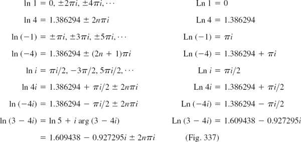

Fig. 337. Some values of ln (3 − 4i) in Example 1
The familiar relations for the natural logarithm continue to hold for complex values, that is,
![]()
but these relations are to be understood in the sense that each value of one side is also contained among the values of the other side; see the next example.
EXAMPLE 2 Illustration of the Functional Relation (5) in Complex
Let
![]()
If we take the principal values
![]()
then (5a) holds provided we write ln (z1z2) = ln 1 = 2πi; however, it is not true for the principal value, Ln (z1z2) = Ln 1 = 0.
THEOREM 1 Analyticity of the Logarithm
For every n = 0, ±1, ±2, … formula (3) defines a function, which is analytic, except at 0 and on the negative real axis, and has the derivative

PROOF
We show that the Cauchy–Riemann equations are satisfied. From (1)–(3) we have

where the constant c is a multiple of 2π. By differentiation,

Hence the Cauchy–Riemann equations hold. [Confirm this by using these equations in polar form, which we did not use since we proved them only in the problems (to Sec. 13.4).] Formula (4) in Sec. 13.4 now gives (6),

Each of the infinitely many functions in (3) is called a branch of the logarithm. The negative real axis is known as a branch cut and is usually graphed as shown in Fig. 338. The branch for n = 0 is called the principal branch of ln z.

General Powers
General powers of a complex number z = x + iy are defined by the formula

Since ln z is infinitely many-valued, zc will, in general, be multivalued. The particular value
![]()
is called the principal value of zc.
If c = n = 1, 2, …, then zn is single-valued and identical with the usual nth power of z.
If c = −1, −2, …, the situation is similar.
If c = 1/n, where n = 2, 3, …, then
![]()
the exponent is determined up to multiples of 2πi/n and we obtain the n distinct values of the nth root, in agreement with the result in Sec. 13.2. If c = p/q, the quotient of two positive integers, the situation is similar, and zc has only finitely many distinct values. However, if c is real irrational or genuinely complex, then zc is infinitely many-valued.

All these values are real, and the principal value (n = 0) is e−π/2.
Similarly, by direct calculation and multiplying out in the exponent,
It is a convention that for real positive z = x the expression zc means eclnx where ln x is the elementary real natural logarithm (that is, the principal value Ln z (z = x > 0) in the sense of our definition). Also, if z = e, the base of the natural logarithm, zc = ec is conventionally regarded as the unique value obtained from (1) in Sec. 13.5.
From (7) we see that for any complex number a,

We have now introduced the complex functions needed in practical work, some of them (ez, cos z, sin z, cosh z, sinh z) entire (Sec. 13.5), some of them (tan z, cot z, tanh z, coth z) analytic except at certain points, and one of them (ln z) splitting up into infinitely many functions, each analytic except at 0 and on the negative real axis.
For the inverse trigonometric and hyperbolic functions see the problem set.
1–4 VERIFICATIONS IN THE TEXT
- Verify the computations in Example 1.
- Verify (5) for z1 = −1 and z2 = −1.
- Prove analyticity of Ln z by means of the Cauchy–Riemann equations in polar form (Sec. 13.4).
- Prove (4a) and (4b).
COMPLEX NATURAL LOGARITHM ln z
5–11 Principal Value Ln z. Find Ln z when z equals
- 5. −11
- 6. 4 + 4i
- 7. 4 − 4i
- 8. 1 ± i
- 9. 0.6 + 0.8i
- 10. −15 ± 0.1i
- 11. ei
12–16 All Values of lnz. Find all values and graph some of them in the complex plane.
- 12. ln e
- 13. ln 1
- 14. ln (−7)
- 15. ln (ei)
- 16. ln (4 + 3i)
- 17. Show that the set of values of ln(i2) differs from the set of values of 2 ln i.
18–21 Equations. Solve for z.
- 18. ln z = −πi/2
- 19. ln z = 4 − 3i
- 20. ln z = e − πi
- 21. ln z = 0.6 + 0.4i
22–28 General Powers. Find the principal value. Show details.
- 22. (2i)2i
- 23. (1 + i)1−i
- 24. (1 − i)1+i
- 25. (−3)3−i
- 26. (i)i/2
- 27. (−1)2−i
- 28. (3 + 4i)1/3
- 29. How can you find the answer to Prob. 24 from the answer to Prob. 23?
- 30. TEAM PROJECT. Inverse Trigonometric and Hyperbolic Functions. By definition, the inverse sine w = arcsin z is the relation such that sin w = z. The inverse cosine w = arccos z is the relation such that cos w = z. The inverse tangent, inverse cotangent, inverse hyperbolic sine, etc., are defined and denoted in a similar fashion. (Note that all these relations are multivalued.) Using sin w = (eiw − e−iw)/(2i) and similar representations of cos w, etc., show that


- Show that w = arcsin z is infinitely many-valued, and if w1 is one of these values, the others are of the form and w1 ± 2nπ and π −w1 ± 2nπ, n = 0, 1, …. (The principal value of w = u + iv = arcsin z is defined to be the value for which −π/2 u π/2 if v 0 and −π/2 < u < π/2 if v < 0.)
CHAPTER 13 REVIEW QUESTIONS AND PROBLEMS
- Divide 15 + 23i by −3 + 7i. Check the result by multiplication.
- What happens to a quotient if you take the complex conjugates of the two numbers? If you take the absolute values of the numbers?
- Write the two numbers in Prob. 1 in polar form. Find the principal values of their arguments.
- State the definition of the derivative from memory. Explain the big difference from that in calculus.
- What is an analytic function of a complex variable?
- Can a function be differentiable at a point without being analytic there? If yes, give an example.
- State the Cauchy–Riemann equations. Why are they of basic importance?
- Discuss how ez, cos z, sin z, cosh z, sinh z are related.
- ln z is more complicated than ln x. Explain. Give examples.
- How are general powers defined? Give an example. Convert it to the form x + iy.
11–16 Complex Numbers. Find, in the form x + iy, showing details,
- 11. (2 + 3i)2
- 12. (1 −i)10
- 13. 1/(4 + 3i)
- 14.

- 15. (1 + i)/(1 − i)
- 16. eπi/2, e−πi/2
17–20 Polar Form. Represent in polar form, with the principal argument.
- 17. −4 − 4i
- 18. 12 + i, 12 − i
- 19. −15i
- 20. 0.6 + 0.8i
21–24 Roots. Find and graph all values of:
- 21.

- 22.

- 23.

- 24.

25–30 Analytic Functions. Find f(z) = u(x, y) + iv(x, y) with u or v as given. Check by the Cauchy–Riemann equations for analyticity.
- 25 u = xy
- 26. v = y/(x2 + y2)
- 27. v = −e−2x sin 2y
- 28. u = cos 3x cosh 3y
- 29. u = exp(−(x2 − y2)/2) cos xy
- 30. v = cos 2x sinh 2y
31–35 Special Function Values. Find the value of:
- 31. cos (3 − i)
- 32. Ln (0.6 + 0.8i)
- 33. tan i
- 34. sinh (1 + πi), sin(1 + πi)
- 35. cosh (π + πi)
SUMMARY OF CHAPTER 13 Complex Numbers and Functions. Complex Differentiation
For arithmetic operations with complex numbers
![]()
![]() θ = arctan (y/x), and for their representation in the complex plane, see Secs. 13.1 and 13.2.
θ = arctan (y/x), and for their representation in the complex plane, see Secs. 13.1 and 13.2.
A complex function f(z) = u(x, y) + iv(x, y) is analytic in a domain D if it has a derivative (Sec. 13.3)

everywhere in D. Also, f(z) is analytic at a point z = z0 if it has a derivative in a neighborhood of z0 (not merely at z0 itself).
If f(z) is analytic in D, then u(x, y) and v(x, y) satisfy the (very important!) Cauchy–Riemann equations (Sec. 13.4)

everywhere in D. Then u and v also satisfy Laplace's equation
![]()
everywhere in D. If u(x, y) and v(x, y) are continuous and have continuous partial derivatives in D that satisfy (3) in D, then f(z) = u(x, y) + iv(x, y) is analytic in D. See Sec. 13.4. (More on Laplace's equation and complex analysis follows in Chap. 18.)
The complex exponential function (Sec. 13.5)
![]()
reduces to ex if z = x(y = 0). It is periodic with 2πi and has the derivative ez.
The trigonometric functions are (Sec. 13.6)

and, furthermore,
![]()
The hyperbolic functions are (Sec. 13.6)
![]()
etc. The functions (5)–(7) are entire, that is, analytic everywhere in the complex plane.
The natural logarithm is (Sec. 13.7)
![]()
where z ≠ 0 and n = 0, 1, …. Arg z is the principal value of arg z, that is, −π < Arg z ![]() π. We see that ln z is infinitely many-valued. Taking n = 0 gives the principal value Ln z of ln z; thus Ln z = ln|z| + i Arg z.
π. We see that ln z is infinitely many-valued. Taking n = 0 gives the principal value Ln z of ln z; thus Ln z = ln|z| + i Arg z.
General powers are defined by (Sec. 13.7)
![]()
1First to use complex numbers for this purpose was the Italian mathematician GIROLAMO CARDANO (1501–1576), who found the formula for solving cubic equations. The term “complex number” was introduced by CARL FRIEDRICH GAUSS (see the footnote in Sec. 5.4), who also paved the way for a general use of complex numbers.
2Sometimes called the Argand diagram, after the French mathematician JEAN ROBERT ARGAND (1768–1822), born in Geneva and later librarian in Paris. His paper on the complex plane appeared in 1806, nine years after a similar memoir by the Norwegian mathematician CASPAR WESSEL (1745–1818), a surveyor of the Danish Academy of Science.
3 ABRAHAM DE MOIVRE (1667–1754), French mathematician, who pioneered the use of complex numbers in trigonometry and also contributed to probability theory (see Sec. 24.8).
4The French mathematician AUGUSTIN-LOUIS CAUCHY (see Sec. 2.5) and the German mathematicians BERNHARD RIEMANN (1826–1866) and KARL WEIERSTRASS (1815–1897; see also Sec. 15.5) are the founders of complex analysis. Riemann received his Ph.D. (in 1851) under Gauss (Sec. 5.4) at Göttingen, where he also taught until he died, when he was only 39 years old. He introduced the concept of the integral as it is used in basic calculus courses, and made important contributions to differential equations, number theory, and mathematical physics. He also developed the so-called Riemannian geometry, which is the mathematical foundation of Einstein's theory of relativity; see Ref. [GenRef9] in App. 1.