THEOREM 1 Fundamental Theorem for the Homogeneous Linear ODE (2)

For a homogeneous linear ODE (2), sums and constant multiples of solutions on some open interval I are again solutions on I. (This does not hold for a nonhomogeneous or nonlinear ODE!)

DEFINITION General Solution, Basis, Particular Solution

A general solution of (2) on an open interval I is a solution of (2) on I of the form

where y₁, …, y_n is a basis (or fundamental system) of solutions of (2) on I; that is, these solutions are linearly independent on I, as defined below.

A particular solution of (2) on I is obtained if we assign specific values to the n constants c₁, …, c_n in (3).

DEFINITION Linear Independence and Dependence

Consider n functions y₁(x), …, y_n(x) defined on some interval I.

These functions are called linearly independent on I if the equation

implies that all k₁, …, k_n are zero. These functions are called linearly dependent on I if this equation also holds on I for some k₁, …, k_n not all zero.

EXAMPLE 1 Linear Dependence

Show that the functions y₁ = x², y₂ = 5x, y₃ = 2x are linearly dependent on any interval.

Solution.. y₂ = 0y₁ + 2.5y₃. This proves linear dependence on any interval.

EXAMPLE 2 Linear Independence

Show that y₁ = x, y₂ = x², y₃ = x³ are linearly independent on any interval, for instance, on −1 x 2.

Solution. Equation (4) is k₁x + k₂x² + k₃x³ = 0. Taking (a) x = −1, (b) x = 1, (c) x =2, we get

k₂ = 0 from (a) + (b). Then k₃ = 0 from (c) −2(b). Then k₁ = 0 from (b). This proves linear independence.

A better method for testing linear independence of solutions of ODEs will soon be explained.

EXAMPLE 3 General Solution. Basis

Solve the fourth-order ODE

Solution. As in Sec. 2.2 we substitute y = e^λx. Omitting the common factor e^λx, we obtain the characteristic equation

This is a quadratic equation in ν = λ² namely,

The roots are ν = 1 and 4. Hence λ = −2, −1, 1, 2. This gives four solutions. A general solution on any interval is

provided those four solutions are linearly independent. This is true but will be shown later.

THEOREM 2 Existence and Uniqueness Theorem for Initial Value Problems

If the coefficients p₀(x), …, p_n−1(x) of (2) are continuous on some open interval I and x₀ is in I, then the initial value problem (2), (5) has a unique solution y(x) on I.

EXAMPLE 4 Initial Value Problem for a Third-Order Euler–Cauchy Equation

Solve the following initial value problem on any open interval I on the positive x-axis containing x = 1.

Solution. Step 1. General solution. As in Sec. 2.5 we try y = x^m. By differentiation and substitution,

Dropping x^m and ordering gives m³ − 6m² + 11m − 6 = 0. If we can guess the root m = 1. We can divide by m − 1 and find the other roots 2 and 3, thus obtaining the solutions x, x², x³, which are linearly independent on I (see Example 2). [In general one shall need a root-finding method, such as Newton's (Sec. 19.2), also available in a CAS (Computer Algebra System).] Hence a general solution is

valid on any interval I, even when it includes x = 0 where the coefficients of the ODE divided by x³ (to have the standard form) are not continuous.

Step 2. Particular solution. The derivatives are y′ = c₁ = 2c₂x + 3c₃x² and y″ = 2c₂ + 6c₃x. From this, and y and the initial conditions, we get by setting x = 1

This is solved by Cramer's rule (Sec. 7.6), or by elimination, which is simple, as follows. (b) − (a) gives (d) c₂ + 2c₃ = −1. Then (c) − 2(d) gives c₃ = −1. Then (c) gives c₂ = 1. Finally c₁ = 2 from (a). Answer: y = 2x + x² − x³.

THEOREM 3 Linear Dependence and Independence of Solutions

Let the ODE (2) have continuous coefficients p₀(x), …, p_x−1(x) on an open interval I. Then n solutions y₁, …, y_n of (2) on I are linearly dependent on I if and only if their Wronskian is zero for some x = x₀ in I. Furthermore, if W is zero for x = x₀, then W is identically zero on I. Hence if there is an x₁ in I at which W is not zero, then y₁, …, y_n are linearly independent on I, so that they form a basis of solutions of (2) on I.

PROOF

(a) Let y₁, …, y_n be linearly dependent solutions of (2) on I. Then, by definition, there are constants k₁, …, k_n not all zero, such that for all x in I,

By n − 1 differentiations of (7) we obtain for all x in I

(7), (8) is a homogeneous linear system of algebraic equations with a nontrivial solution k₁, …, k_n. Hence its coefficient determinant must be zero for every x on I, by Cramer's theorem (Sec. 7.7). But that determinant is the Wronskian W, as we see from (6). Hence W is zero for every x on I.

(b) Conversely, if W is zero at an x₀ in I, then the system (7), (8) with x = x₀ has a solution not all zero, by the same theorem. With these constants we define the solution of (2) on I. By (7), (8) this solution satisfies the initial conditions . But another solution satisfying the same conditions is y ≡ 0. Hence y* ≡ y by Theorem 2, which applies since the coefficients of (2) are continuous. Together, on I. This means linear dependence of y₁, …, y_n on I.

(c) If W is zero at an x₀ in I, we have linear dependence by (b) and then W ≡ 0 by (a). Hence if W is not zero at an x₁ in I, the solutions y₁, …, y_n must be linearly independent on I.

EXAMPLE 5 Basis, Wronskian

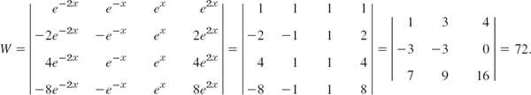
We can now prove that in Example 3 we do have a basis. In evaluating W, pull out the exponential functions columnwise. In the result, subtract Column 1 from Columns 2, 3, 4 (without changing Column 1). Then expand by Row 1. In the resulting third-order determinant, subtract Column 1 from Column 2 and expand the result by Row 2:

THEOREM 4 Existence of a General Solution

If the coefficients of p₀(x), …, p_n−1(x) of (2) are continuous on some open interval I, then (2) has a general solution on I.

PROOF

We choose any fixed x₀ in I. By Theorem 2 the ODE (2) has n solutions y₁, …, y_n, where y_j satisfies initial conditions (5) with K_j−1 = 1 and all other K's equal to zero. Their Wronskian at x₀ equals 1. For instance, when n = 3, then y₁(x₀) = 1, , , and the other initial values are zero. Thus, as claimed,

Hence for any n those solutions y₁, …, y_n are are linearly independent on I, by Theorem 3. They form a basis on I, and y = c₁y₁ + … + c_ny_n is a general solution of (2) on I.

THEOREM 5 General Solution Includes All Solutions

If the ODE (2) has continuous coefficients p₀(x), …, p_n−1(x) on some open interval I, then every solution y = Y(x) of (2) on I is of the form

where y₁, …, y_n is a basis of solutions of (2) on I and C₁, …, C_n are suitable constants.

PROOF

Let Y be a given solution and y = c₁y₁ + … + c_ny_n a general solution of (2) on I. We choose any fixed x₀ in I and show that we can find constants c₁, …, c_n for which y and its first n − 1 derivatives agree with Y and its corresponding derivatives at x₀. That is, we should have at x = x₀

But this is a linear system of equations in the unknowns c₁, …, c_n. Its coefficient determinant is the Wronskian W of y₁, …, y_n at x₀. Since y₁, …, y_n form a basis, they are linearly independent, so that W is not zero by Theorem 3. Hence (10) has a unique solution c₁ = C₁, …, c_n = C_n (by Cramer's theorem in Sec. 7.7). With these values we obtain the particular solution

on I. Equation (10) shows that y* and its first n − 1 derivatives agree at x₀ with Y and its corresponding derivatives. That is, y* and Y satisfy, at x₀, the same initial conditions. The uniqueness theorem (Theorem 2) now implies that y* ≡ Y on I. This proves the theorem.

PROBLEM SET 3.1

1–6 BASES: TYPICAL EXAMPLES

To get a feel for higher order ODEs, show that the given functions are solutions and form a basis on any interval. Use Wronskians. In Prob. 6, x > 0,

1. 1, x, x², x³, y^iv = 0
2. e^x, e^−x, e^2x, y″′ − y′ + 2y = 0
3. cos x, sin x, x cos x, x sin x, y^iv + 2y″ + y = 0
4. e^−4x, xe^−4x, x²e^−4x, y″′ + 12y″ + 48y′ + 64y = 0
5. 1, e^−x cos 2x, e^−x sin 2x, y″′ + 2y″ + 5y′ = 0
6. 1, x², x⁴, x²y″ − 3xy″ + 3y′ = 0
7. TEAM PROJECT. General Properties of Solutions of Linear ODEs. These properties are important in obtaining new solutions from given ones. Therefore extend Team Project 38 in Sec. 2.2 to nth-order ODEs. Explore statements on sums and multiples of solutions of (1) and (2) systematically and with proofs. Recognize clearly that no new ideas are needed in this extension from n = 2 to general n.

8–15 LINEAR INDEPENDENCE

Are the given functions linearly independent or dependent on the half-axis x ≥ 0? Give reason.

• 8. x², 1/x², 0
• 9. tan x, cot x, 1
• 10. e^2x, xe^2x, x²e^2x
• 11. e^x cos x, e^x sin x, e^x
• 12. sin² x, cos² x, cos 2x
• 13. sin x, cos x, sin 2x
• 14. cos² x, sin² x, 2π
• 15. cosh 2x, sinh 2x, e^2x
• 16. TEAM PROJECT. Linear Independence and Dependence. (a) Investigate the given question about a set S of functions on an interval I. Give an example. Prove your answer.

  (1) If S contains the zero function, can S be linearly independent?

  (2) If S is linearly independent on a subinterval J of I, is it linearly independent on I?

  (3) If S is linearly dependent on a subinterval J of I, is it linearly dependent on I?

  (4) If S is linearly independent on I, is it linearly independent on a subinterval J?

  (5) If S is linearly dependent on I, is it linearly independent on a subinterval J?

  (6) If S is linearly dependent on I, and if T contains S, is T linearly dependent on I?

  (b) In what cases can you use the Wronskian for testing linear independence? By what other means can you perform such a test?

EXAMPLE 1 Distinct Real Roots

Solve the ODE y″′ − 2y″ − y′ + 2y = 0.

Solution. The characteristic equation is λ³ − 2λ² − λ + 2 = 0. It has the roots −1, 1, 2; if you find one of them by inspection, you can obtain the other two roots by solving a quadratic equation (explain!). The corresponding general solution (4) is y = c₁e^−x + c₂e^x + c₃e^2x.

THEOREM 1 Basis

Solutions of (1) (with any real or complex λ_j's) form a basis of solutions of (1) on any open interval if and only if all n roots of (2) are different.

THEOREM 2 Linear Independence

Any number of solutions of (1) of the form e^λx are linearly independent on an open interval I if and only if the corresponding λ are all different.

EXAMPLE 2 Simple Complex Roots. Initial Value Problem

Solve the initial value problem

Solution. The characteristic equation is λ³ − λ² + 100λ − 100 = 0. It has the root 1, as can perhaps be seen by inspection. Then division by λ − 1 shows that the other roots are ±10i Hence a general solution and its derivatives (obtained by differentiation) are

From this and the initial conditions we obtain, by setting x = 0,

We solve this system for the unknowns A, B, c₁. Equation (a) minus Equation (c) gives 101A = 303, A = 3. Then c₁ = 1 from (a) and B = 1 from (b). The solution is (Fig. 73)

This gives the solution curve, which oscillates about e^x (dashed in Fig. 73).

EXAMPLE 3 Real Double and Triple Roots

Solve the ODE y^ν − 3y^iv + 3y″′ − y″ = 0.

Solution. The characteristic equation λ⁵ − 3λ⁴ + 3λ³ − λ² = 0 has the roots λ₁ = λ₂ = 0, and λ₃ = λ₄ = λ₅ = 1, and the answer is

PROBLEM SET 3.2

1–6 GENERAL SOLUTION

Solve the given ODE. Show the details of your work.

1. y″′ + 25y′ = 0
2. y^iv + 2y″ + y = 0
3. y^iv + 4y″ = 0
4. (D³ − D² − D + I)y = 0
5. (D⁴ + 10D² + 9I)y = 0
6. (D⁵ + 8D³ + 16D)y = 0

7–13 INITIAL VALUE PROBLEM

Solve the IVP by a CAS, giving a general solution and the particular solution and its graph.

• 7. y″′ + 3.2y″ + 4.81y′ = 0, y(0) = 3.4, y′(0) = −4.6, y″(0) = 9.91
• 8. y″′ + 7.5y″ + 14.25y′ − 9.125y = 0, y(0) = 10.05, y′(0) = −54.975, y″(0) = 257.5125
• 9. 4y″′ + 8y″ + 41y′ + 37y = 0, y(0) = 9, y′(0) = −6.5, y″(0) = −39.75
• 10.
• 11. y^iv − 9y″ − 400y = 0, y(0) = 0, y′(0) = 0, y″ = 41, y″′(0) = 0
• 12. y^v − 5y″′ + 4y′ = 0, y(0) = 3, y′(0) = −5, y″(0) = 11, y″′(0) = −23, y^iv(0) = 47
• 13. y^iv + 0.45y″′ − 0.165y″ + 0.0045y′ − 0.00175y = 0, y(0) = 17.4, y′(0) = −2.82, y″(0) = 2.0485, y″′(0) = −1.458675
• 14. PROJECT. Reduction of Order. This is of practical interest since a single solution of an ODE can often be guessed. For second order, see Example 7 in Sec. 2.1.

  (a) How could you reduce the order of a linear constant-coefficient ODE if a solution is known?

  (b) Extend the method to a variable-coefficient ODE

  

  Assuming a solution y₁ to be known, show that another solution is y₂(x) = u(x)y₁(x) with u(x) = ∫z(x) dx and z obtained by solving

  

  (c) Reduce

  

  using y₁ = x (perhaps obtainable by inspection).

• 15. CAS EXPERIMENT. Reduction of Order. Starting with a basis, find third-order linear ODEs with variable coefficients for which the reduction to second order turns out to be relatively simple.

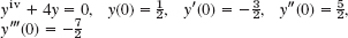
EXAMPLE 1 Initial Value Problem. Modification Rule

Solve the initial value problem

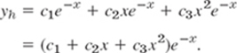
Solution. Step 1. The characteristic equation is λ³ + 3λ² + 3λ + 1 = (λ + 1)³ = 0. It has the triple root λ = −1. Hence a general solution of the homogeneous ODE is

Step 2. If we try y_p = Ce^−x, we get −C + 3C − 3C + C = 30, which has no solution. Try Cxe^−x and Cx²e^−x. The Modification Rule calls for

Substitution of these expressions into (6) and omission of the common factor e^−x gives

The linear, quadratic, and cubic terms drop out, and 6C = 30. Hence C = 5. This gives y_p = 5x³e^−x.

Step 3. We now write down y = y_h + y_p, the general solution of the given ODE. From it we find c₁ by the first initial condition. We insert the value, differentiate, and determine c₂ from the second initial condition, insert the value, and finally determine c₃ from y″(0) and the third initial condition:

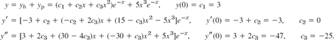
Hence the answer to our problem is (Fig. 73)

The curve of y begins at (0, 3) with a negative slope, as expected from the initial values, and approaches zero as x → ∞. The dashed curve in Fig. 74 is y_p.

EXAMPLE 2 Variation of Parameters. Nonhomogeneous Euler–Cauchy Equation

Solve the nonhomogeneous Euler–Cauchy equation

Solution. Step 1. General solution of the homogeneous ODE. Substitution of y = x^m and the derivatives into the homogeneous ODE and deletion of the factor x^m gives

The roots are 1, 2, 3 and give as a basis

Hence the corresponding general solution of the homogeneous ODE is

Step 2. Determinants needed in (7). These are

Step 3. Integration. In (7) we also need the right side r(x) of our ODE in standard form, obtained by division of the given equation by the coefficient x³ of y″′; thus, r(x) = (x⁴ ln x)/x³ = x ln x. In (7) we have the simple quotients W₁/W = x/2, W₂/W = −1, W₃/W = 1/(2x). Hence (7) becomes

Simplification gives . Hence the answer is

Figure 75 shows Can you explain the shape of this curve? Its behavior near x = 0? The occurrence of a minimum? Its rapid increase? Why would the method of undetermined coefficients not have given the solution?

EXAMPLE 3 Bending of an Elastic Beam under a Load

We consider a beam B of length L and constant (e.g., rectangular) cross section and homogeneous elastic material (e.g., steel); see Fig. 76. We assume that under its own weight the beam is bent so little that it is practically straight. If we apply a load to B in a vertical plane through the axis of symmetry (the x-axis in Fig. 76), B is bent. Its axis is curved into the so-called elastic curve C (or deflection curve). It is shown in elasticity theory that the bending moment M(x) is proportional to the curvature k(x) of C. We assume the bending to be small, so that the deflection y(x) and its derivative y′(x) (determining the tangent direction of C) are small. Then, by calculus, k = y″/(1 + y′²)^3/2 ≈ y″. Hence

EI is the constant of proportionality. E is Young's modulus of elasticity of the material of the beam. I is the moment of inertia of the cross section about the (horizontal) z-axis in Fig. 76.

Elasticity theory shows further that M″ (x) = f(x), where f(x) is the load per unit length. Together,

Fig. 76. Elastic beam

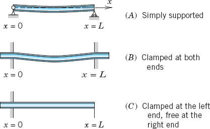
In applications the most important supports and corresponding boundary conditions are as follows and shown in Fig. 77.

The boundary condition y = 0 means no displacement at that point, y′ = 0 means a horizontal tangent, y″ = 0 means no bending moment, and y″′ = 0 means no shear force.

Let us apply this to the uniformly loaded simply supported beam in Fig. 76. The load is f(x) ≡ f₀ = const. Then (8) is

This can be solved simply by calculus. Two integrations give

y″(0) = 0 gives c₂ = 0. Then (since L ≠ 0). Hence

Integrating this twice, we obtain

with c₄ = 0 from y(0) = 0. Then

Inserting the expression for k, we obtain as our solution

Since the boundary conditions at both ends are the same, we expect the deflection y(x) to be “symmetric” with respect to L/2, that is, y(x) = y(L − x). Verify this directly or set x = u + L/2 and show that y becomes an even function of u,

From this we can see that the maximum deflection in the middle at u = 0(x = L/2) is 5f₀L⁴/(16 · 24EI). Recall that the positive direction points downward.

PROBLEM SET 3.3

1–7 GENERAL SOLUTION

Solve the following ODEs, showing the details of your work.

1. y″′ + 3y″ + 3y′ + y = e^x − x − 1
2. y″′ + 2y″ − y′ − 2y = 1 − 4x³
3. (D⁴ + 10D² + 9I)y = 6.5 sinh 2x
4. (D³ + 3D² − 5D − 39I)y = −300 cos x
5. (x³D³ + x²D² − 2xD + 2I)y = x⁻²
6. (D³ + 4D)y = sin x
7. (D³ − 9D² + 27D − 27I)y = 27 sin 3x

8–13 INITIAL VALUE PROBLEM

Solve the given IVP, showing the details of your work.

• 8. y^iv − 5y″ + 4y = 10e^−3x, y(0) = 1, y′(0) = 0, y′(0) = 0, y″′(0) = 0
• 9. y^iv + 5y″ + 4y = 90 sin 4x, y(0) = 1, y′(0) = 2, y″(0) = −1, y″′(0) = −32
• 10. x³y″′ + xy′ − y = x², y(1) = 1, y′(1) = 3, y″(1) = 14
• 11. (D³ − 2D² − 3D)y = 74e^−3x sin x, y(0) = −1.4, y′(0) = 3.2, y″(0) = −5.2
• 12. (D³ − 2D² − 9D + 18I)y = e^2x, y(0) = 4.5, y′(0) = 8.8, y″(0) = 17.2
• 13. (D³ − 4D)y = 10 cos x + 5 sin x, y(0) = 3, y′(0) = −2, y″(0) = −1
• 14. CAS EXPERIMENT. Undetermined Coefficients. Since variation of parameters is generally complicated, it seems worthwhile to try to extend the other method. Find out experimentally for what ODEs this is possible and for what not. Hint: Work backward, solving ODEs with a CAS and then looking whether the solution could be obtained by undetermined coefficients. For example, consider

  

  and

  

• 15. WRITING REPORT. Comparison of Methods. Write a report on the method of undetermined coefficients and the method of variation of parameters, discussing and comparing the advantages and disadvantages of each method. Illustrate your findings with typical examples. Try to show that the method of undetermined coefficients, say, for a third-order ODE with constant coefficients and an exponential function on the right, can be derived from the method of variation of parameters.

Compare with the similar Summary of Chap. 2 (the case n = 2).

Chapter 3 extends Chap. 2 from order n = 2 to arbitrary n. An nth-order linear ODE is an ODE that can be written

with y⁽ⁿ⁾ = dⁿy/dxⁿ as the first term; we again call this the standard form. Equation (1) is called homogeneous if r(x) ≡ 0 on a given open interval I considered, nonhomogeneous if r(x) 0 on I. For the homogeneous ODE

the superposition principle (Sec. 3.1) holds, just as in the case n = 2. A basis or fundamental system of solutions of (2) on I consists of n linearly independent solutions y₁, … y_n of (2) on I. A general solution of (2) on I is a linear combination of these,

A general solution of the nonhomogeneous ODE (1) on I is of the form

Here, y_p is a particular solution of (1) and is obtained by two methods (undetermined coefficients or variation of parameters) explained in Sec. 3.3.

An initial value problem for (1) or (2) consists of one of these ODEs and n initial conditions (Secs. 3.1, 3.3)

with given x₀ in I and given K₀, …, K_n−1. If p₀, …, p_n−1, r are continuous on I, then general solutions of (1) and (2) on I exist, and initial value problems (1), (5) or (2), (5) have a unique solution.